Chapter 8 S’more Hypothesis Testing
In Chapter 7,
we introduced a framework for hypothesis testing using verbs
from the package infer,
and demonstrated it within the context of
testing difference between proprotions.
In this chapter, we continue to demonstrate this framework
by applying it to another type of problems: testing difference between means.
We will walk you through two examples,
each one twice, once with the infer-based simulation method,
followed by the traditional theory-based method.
Needed packages
Let’s get ready all the packages we will need for this chapter.
# Install xfun so that I can use xfun::pkg_load2
if (!requireNamespace('xfun')) install.packages('xfun')
xf <- loadNamespace('xfun')

cran_packages <- c(
                  "dplyr",
                  "ggplot2",
                  "infer",
                  "moderndive",
                  "skimr",
                  "tibble",
                  "tidyr"
)

if (length(cran_packages) != 0) xf$pkg_load2(cran_packages)

gg <- import::from(ggplot2, .all=TRUE, .into={new.env()})
dp <- import::from(dplyr, .all=TRUE, .into={new.env()})

import::from(magrittr, "%>%")
import::from(patchwork, .all=TRUE)
8.1 Example 1
Are action or romance movies rated higher?
Let’s apply our knowledge of hypothesis testing to answer the question: “Are action or romance movies rated higher on IMDb?” IMDb is a database on the internet providing information on movie and television show casts, plot summaries, trivia, and user ratings. We’ll investigate whether, on average, action or romance movies get higher ratings on IMDb.
8.1.1 IMDb ratings data
The movies_sample dataset in the moderndive package
is a random sample of 68 movies that are classified
as either “action” or “romance” but not both.
# A tibble: 68 x 4
   title                     year rating genre
   <chr>                    <int>  <dbl> <chr>
 1 Underworld                1985    3.1 Action
 2 Love Affair               1932    6.3 Romance
 3 Junglee                   1961    6.8 Romance
 4 Eversmile, New Jersey     1989    5   Romance
 5 Search and Destroy        1979    4   Action
 6 Secreto de Romelia, El    1988    4.9 Romance
 7 Amants du Pont-Neuf, Les  1991    7.4 Romance
 8 Illicit Dreams            1995    3.5 Action
 9 Kabhi Kabhie              1976    7.7 Romance
10 Electric Horseman, The    1979    5.8 Romance
# … with 58 more rows
The variables include the title and year the movie was filmed.
Furthermore, we have a numerical variable rating,
which is the IMDb rating out of 10 stars,
and a binary categorical variable genre indicating
if the movie was an Action or Romance movie.
We are interested in whether Action or Romance movies
got a higher rating on average.
Let’s perform an exploratory data analysis of this data. Recall from Subsection 2.7.1 that a boxplot is a visualization we can use to show the relationship between a numerical and a categorical variable.
gg$ggplot(data = movies_sample, gg$aes(x = genre, y = rating)) +
  gg$geom_boxplot() +
  gg$labs(y = "IMDb rating")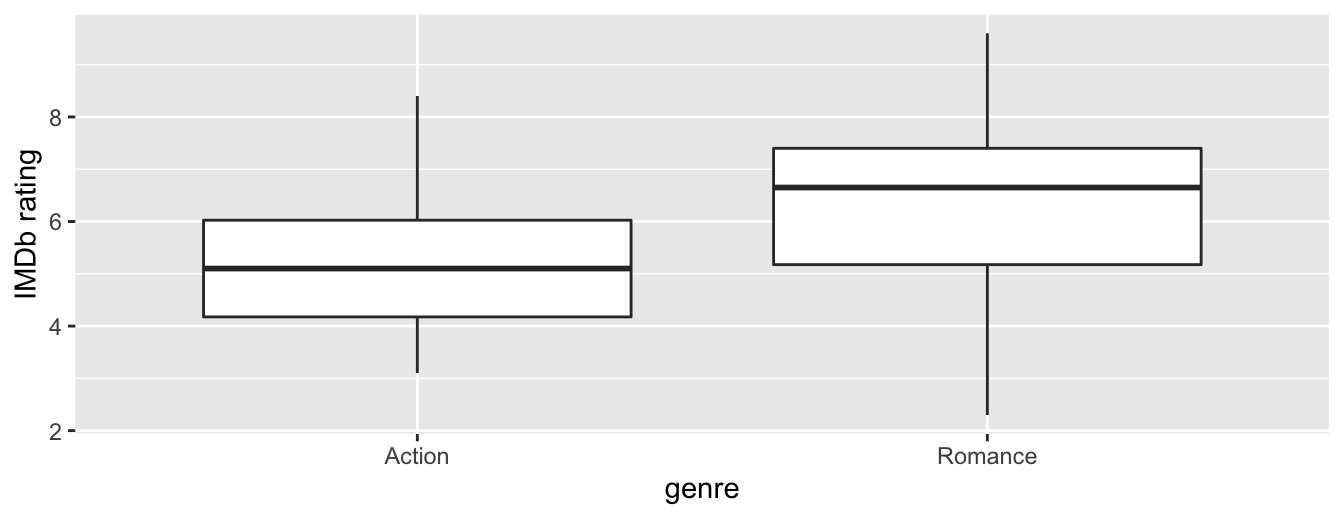
Figure 8.1: Boxplot of IMDb rating vs. genre.
Eyeballing Figure 8.1, romance movies have a higher median rating. Do we have reason to believe, however, that there is a significant difference between the mean rating for action movies compared to romance movies? It’s hard to say just based on this plot. The boxplot does show that the median sample rating is higher for romance movies.
However, there is a large amount of overlap between the boxes. Recall that the median isn’t necessarily the same as the mean either, depending on whether the distribution is skewed.
Let’s calculate some summary statistics split by the binary categorical variable genre: the number of movies, the mean rating, and the standard deviation split by genre. We’ll do this using dplyr data wrangling verbs. Notice in particular how we count the number of each type of movie using the n() summary function.
movies_sample %>%
  dp$group_by(genre) %>%
  dp$summarize(n = dp$n(), mean_rating = mean(rating), std_dev = sd(rating))
# A tibble: 2 x 4
genre n mean_rating std_dev
* <chr> <int> <dbl> <dbl>
1 Action 32 5.28 1.36
2 Romance 36 6.32 1.61Observe that we have 36 movies with an average rating of 6.32 stars and 32 movies with an average rating of 5.28 stars. The difference in these average ratings is thus 6.32 - 5.28 = 1.05. So there appears to be an edge of 1.05 stars in favor of romance movies. The question is, however, are these results indicative of a true difference for all romance and action movies? Or could we attribute this difference to chance sampling variation?
8.1.2 Sampling scenario
Let’s now revisit this study in terms of terminology and notation
related to sampling we studied in Subsection 5.2.2.
The study population is all movies in the IMDb database
that are either action or romance (but not both).
The sample from this population is the 68 movies
included in the movies_sample dataset.
Since this sample was randomly taken from the population movies,
it is representative of all romance and action movies on IMDb.
Thus, any analysis and results based on movies_sample
can generalize to the entire population.
What are the relevant population parameter and point estimates?
We introduce the fourth sampling scenario in Table 7.3.
| Scenario | Population Parameter | Notation | Point estimate | Symbol(s) |
|---|---|---|---|---|
| 1 | Population proportion | \(p\) | Sample proportion | \(\widehat{p}\) |
| 2 | Population mean | \(\mu\) | Sample mean | \(\widehat{\mu}\) or \(\bar{x}\) |
| 3 | Difference in population proportions | \(p_1 - p_2\) | Difference in sample proportions | \(\widehat{p}_1 - \widehat{p}_2\) |
| 4 | Difference in population means | \(\mu_1 - \mu_2\) | Difference in sample means | \(\bar{x}_1 - \bar{x}_2\) |
| 5 | Population regression slope | \(\beta_1\) | Fitted regression slope | \(\widehat{\beta}_1\) or \(b_1\) |
The banana exercise in Chapter 6 concerned means, and the promotions activity in Chapter 7 concerned differences in proportions. We are now concerned with differences in means.
In other words, the population parameter of interest is the difference in population mean ratings \(\mu_a - \mu_r\), where \(\mu_a\) is the mean rating of all action movies on IMDb and similarly \(\mu_r\) is the mean rating of all romance movies. Additionally the point estimate/sample statistic of interest is the difference in sample means \(\overline{x}_a - \overline{x}_r\), where \(\overline{x}_a\) is the mean rating of the \(n_a\) = 32 movies in our sample and \(\overline{x}_r\) is the mean rating of the \(n_r\) = 36 in our sample. Based on our earlier exploratory data analysis, our estimate \(\overline{x}_a - \overline{x}_r\) is \(5.28 - 6.32 = -1.05\).
So there appears to be a slight difference of
-1.05 in favor of romance movies.
The question is, however, could this difference of
-1.05
be merely due to chance and sampling variation?
Or are these results indicative of a true difference in mean ratings
for all romance and action movies on IMDb?
To answer this question, we’ll use hypothesis testing.
8.1.3 Conducting hypothesis test with infer
Let’s first apply the simulated-based method to this problem. We’ll be testing:
\[ \begin{aligned} H_0 &: \mu_a - \mu_r = 0\\ \text{vs } H_A&: \mu_a - \mu_r \neq 0 \end{aligned} \]
In other words, the null hypothesis \(H_0\) suggests that both romance and action movies have the same mean rating. This is the “hypothesized universe” we’ll assume is true. On the other hand, the alternative hypothesis \(H_A\) suggests that there is a difference. Unlike the one-sided alternative we used in the promotions exercise \(H_A: p_m - p_f > 0\), we are now considering a two-sided alternative of \(H_A: \mu_a - \mu_r \neq 0\).
We also need to set the significance level, a.k.a. the \(\alpha\) level. Recall that in Chapter 7, we introduced a cut-off value to decide if \(p\)-value is sufficiently small to reject null hypothesis. This value defines the boundary on the null distribution, beyond which are unlikely values, and that if the observed statistic is categorized as among these unlikely values, we reject the null hypothesis.
This cut-off value is known as \(\alpha\) value, and the extreme values on the null distribution, as defined by the \(\alpha\) level, make up what is called the critical region (Figure 8.2). These extreme values in the tail(s) of the null distribution define outcomes that are not consistent with the null hypothesis (\(H_0\)); that is, they are very unlikely to occure if the null hypothesis is true. Whenever the data from a research study produce an observed statistic that lands inside the critical region, we conclude that the data are not consistent with the null hypothesis, and we reject the null hypothesis (Gravetter and Wallnau 2011b).
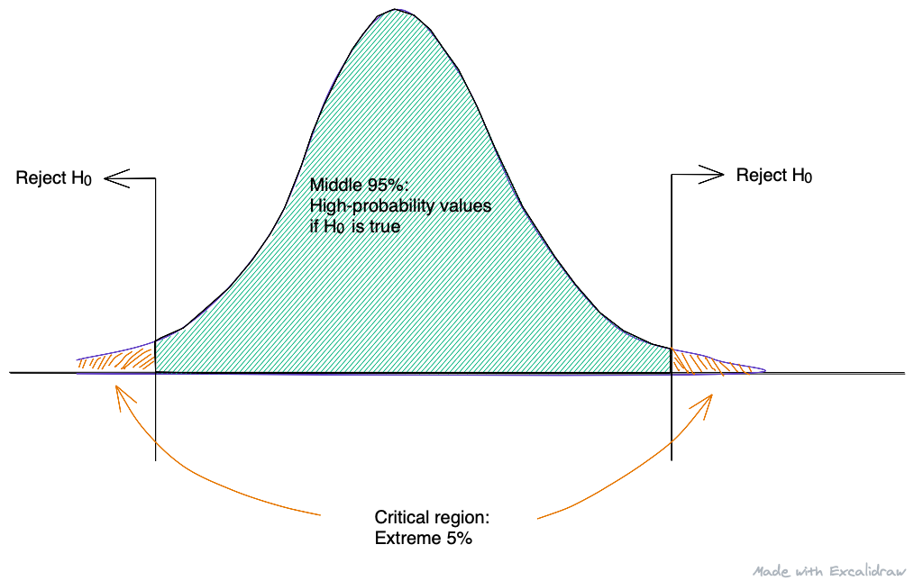
Figure 8.2: critial regions on a sampling distribution for a two-tailed test with \(\alpha = 0.05\).
For the current dataset, we will pre-specify a low significance level of \(\alpha\) = 0.001. By setting this value low, all things being equal, there is a lower chance that the \(p\)-value will be less than \(\alpha\). Thus, there is a lower chance that we’ll reject the null hypothesis \(H_0\) in favor of the alternative hypothesis \(H_A\). In other words, we’ll reject the hypothesis that there is no difference in mean ratings for all action and romance movies, only if we have quite strong evidence. This is known as a “conservative” hypothesis testing procedure.
1. specify variables
Let’s now perform all the steps of the infer workflow. We first specify() the variables of interest in the movies_sample data frame using the formula rating ~ genre. This tells infer that the numerical variable rating is the outcome variable, while the binary variable genre is the explanatory variable. Note that unlike previously when we were interested in proportions, since we are now interested in the mean of a numerical variable, we do not need to set the success argument.
Response: rating (numeric)
Explanatory: genre (factor)
# A tibble: 68 x 2
rating genre
<dbl> <fct>
1 3.1 Action
2 6.3 Romance
3 6.8 Romance
4 5 Romance
5 4 Action
6 4.9 Romance
7 7.4 Romance
8 3.5 Action
9 7.7 Romance
10 5.8 Romance
# … with 58 more rowsObserve at this point that the data in movies_sample has not changed. The only change so far is the newly defined Response: rating (numeric) and Explanatory: genre (factor) meta-data.
2. hypothesize the null
We set the null hypothesis \(H_0: \mu_a - \mu_r = 0\) by using the hypothesize() function. Since we have two samples, action and romance movies, we set null to be "independence" as we described in Section 7.3.
movies_sample %>%
infer::specify(formula = rating ~ genre) %>%
infer::hypothesize(null = "independence")Response: rating (numeric)
Explanatory: genre (factor)
Null Hypothesis: independence
# A tibble: 68 x 2
rating genre
<dbl> <fct>
1 3.1 Action
2 6.3 Romance
3 6.8 Romance
4 5 Romance
5 4 Action
6 4.9 Romance
7 7.4 Romance
8 3.5 Action
9 7.7 Romance
10 5.8 Romance
# … with 58 more rows3. generate replicates
After we have set the null hypothesis, we generate “shuffled” replicates assuming the null hypothesis is true by repeating the shuffling/permutation exercise you performed in Section 7.1.
We’ll repeat this resampling without replacement of type = "permute" a total of reps = 1000 times.
movies_sample %>%
  infer::specify(formula = rating ~ genre) %>%
infer::hypothesize(null = "independence") %>%
infer::generate(reps = 1000, type = "permute")Feel free to run the code below to check out what the generate() step produces.
4. calculate summary statistics
Now that we have 1000 replicated “shuffles” assuming the null hypothesis \(H_0\) that both Action and Romance movies on average have the same ratings on IMDb, let’s calculate() the appropriate summary statistic for these 1000 replicated shuffles. From Section 7.2, summary statistics relating to hypothesis testing have a specific name: test statistics. Since the unknown population parameter of interest is the difference in population means \(\mu_{a} - \mu_{r}\), the test statistic of interest here is the difference in sample means \(\overline{x}_{a} - \overline{x}_{r}\).
For each of our 1000 shuffles, we can calculate this test statistic by setting stat = "diff in means". Furthermore, since we are interested in \(\overline{x}_{a} - \overline{x}_{r}\), we set order = c("Action", "Romance"). Let’s save the results in a data frame called null_distribution_movies:
null_distribution_movies <- movies_sample %>%
  infer::specify(formula = rating ~ genre) %>%
  infer::hypothesize(null = "independence") %>%
  infer::generate(reps = 1000, type = "permute") %>%
  infer::calculate(stat = "diff in means", order = c("Action", "Romance"))
null_distribution_movies
# A tibble: 1,000 x 2
replicate stat
* <int> <dbl>
1 1 0.511
2 2 0.346
3 3 -0.327
4 4 -0.209
5 5 -0.433
6 6 -0.103
7 7 0.387
8 8 0.169
9 9 0.257
10 10 0.334
# … with 990 more rowsObserve that we have 1000 values of stat, each representing one instance of \(\overline{x}_{a} - \overline{x}_{r}\). The 1000 values form the null distribution, which is the technical term for the sampling distribution of the difference in sample means \(\overline{x}_{a} - \overline{x}_{r}\) assuming \(H_0\) is true. What happened in real life? What was the observed difference in promotion rates? What was the observed test statistic \(\overline{x}_{a} - \overline{x}_{r}\)? Recall from our earlier data wrangling, this observed difference in means was \(5.28 - 6.32 = -1.05\). We can also achieve this using the code that constructed the null distribution null_distribution_movies but with the hypothesize() and generate() steps removed. Let’s save this in obs_diff_means:
obs_diff_means <- movies_sample %>%
  infer::specify(formula = rating ~ genre) %>%
  infer::calculate(stat = "diff in means", order = c("Action", "Romance"))
obs_diff_means
# A tibble: 1 x 1
stat
<dbl>
1 -1.055. visualize the p-value
Lastly, in order to compute the \(p\)-value, we have to assess how “extreme” the observed difference in means of -1.05 is. We do this by comparing -1.05 to our null distribution, which was constructed in a hypothesized universe of no true difference in movie ratings. Let’s visualize both the null distribution and the \(p\)-value in Figure 8.3.
Unlike our example in Subsection 7.3.1 involving promotions,
now we have a two-sided \(H_A: \mu_a - \mu_r \neq 0\),
so we set direction = "both".
As a result, the area under the curve
at or more extreme than the observed statistic consists of:
- area to the left of -1.047, and
- area to the right of 1.047
infer::visualize(null_distribution_movies, bins = 10) +
  infer::shade_p_value(obs_stat = obs_diff_means, direction = "both")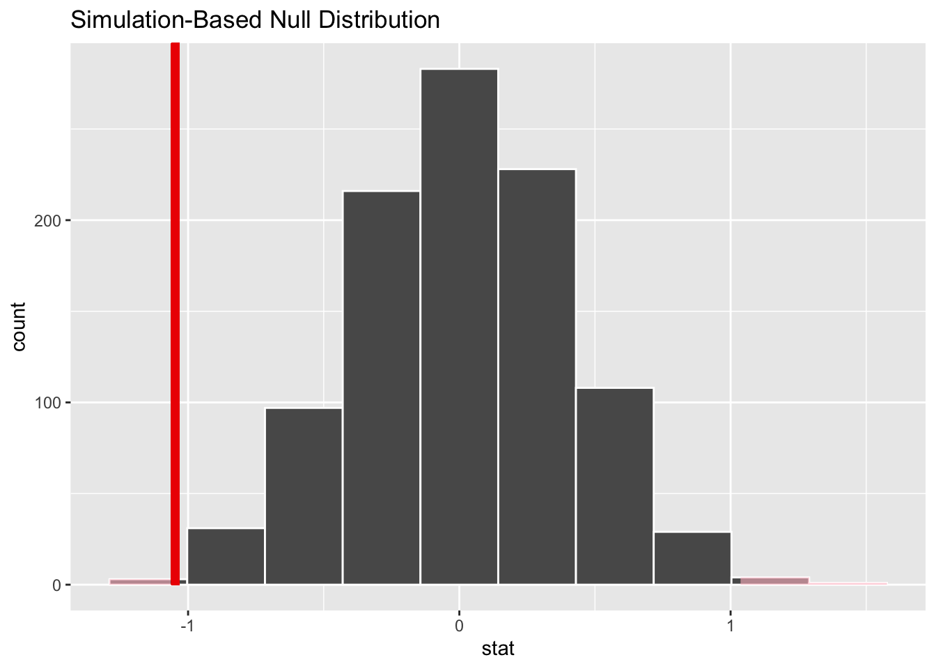
Figure 8.3: Null distribution, observed test statistic, and \(p\)-value.
Let’s go over the elements of this plot. First, the histogram is the null distribution. Second, the solid line is the observed test statistic, or the difference in sample means we observed in real life of \(5.275 - 6.322 = -1.047\). Third, the two shaded areas of the histogram form the \(p\)-value, or the probability of obtaining a test statistic just as or more extreme than the observed test statistic assuming the null hypothesis \(H_0\) is true.
What proportion of the null distribution is shaded? In other words, what is the numerical value of the \(p\)-value? We use the get_p_value() function to compute this value:
# A tibble: 1 x 1
  p_value
    <dbl>
1   0.004
This \(p\)-value of 0.004 is very small, which explains that we can barely discern the shaded region in Figure 8.3 (you may see a pink thin line on either tail if you squint very hard). In other words, there is a very small chance that we would observe a difference of 5.275 - 6.322 = -1.047 in a hypothesized universe where there was truly no difference in ratings.
But this \(p\)-value is larger than our (even smaller) pre-specified \(\alpha\) significance level of 0.001. Thus, we failed to reject the null hypothesis \(H_0: \mu_a - \mu_r = 0\). In non-statistical language, the conclusion is: we do not have the evidence needed in this sample of data to say that romance and action movies in the IMDb are, on average, rated differently.
Learning check
(LC8.1) Conduct the same analysis comparing action movies versus romantic movies using the median rating instead of the mean rating. What was different and what was the same?
(LC8.2)
We visualized the movies_sample using a boxplot
in Figure 8.1.
Another option to do so would be a faceted histogram (see Section 2.6).
Create a faceted histogram for movies_sample.
What conclusions can you make from viewing the faceted histogram
that you couldn’t see when looking at the boxplot?
8.1.4 Theory-based method
Recall that the test statistic we discussed in Section 7.4 for the theory-based method was a \(z\)-statistic, which allowed us to test the difference in two sample proportions. To test the difference between two sample means, we will need to use a different statistic, commonly known as two-sample \(t\)-statistic, and the corresponding theory-based test is a two-sample \(t\)-test.
Check assumptions
Recall that the validity of conclusions drawn from a theory-based method rely on whether assumptions of such method are met. In order to use the two-sample \(t\)-test, we need to check the following assumptions.
Independent observations: The observations are independent in both groups.
Unfortunately, we don’t know how IMDb computes the ratings. For example, if the same person rated multiple movies, then those observations would be related and hence not independent.
Approximately normal: The distribution of the response for each group should be normal or the sample sizes should be at least 30.
movies_sample %>%
  gg$ggplot(gg$aes(x = rating)) +
  gg$geom_histogram(color = "white", binwidth = 1) +
  gg$facet_wrap(~ genre)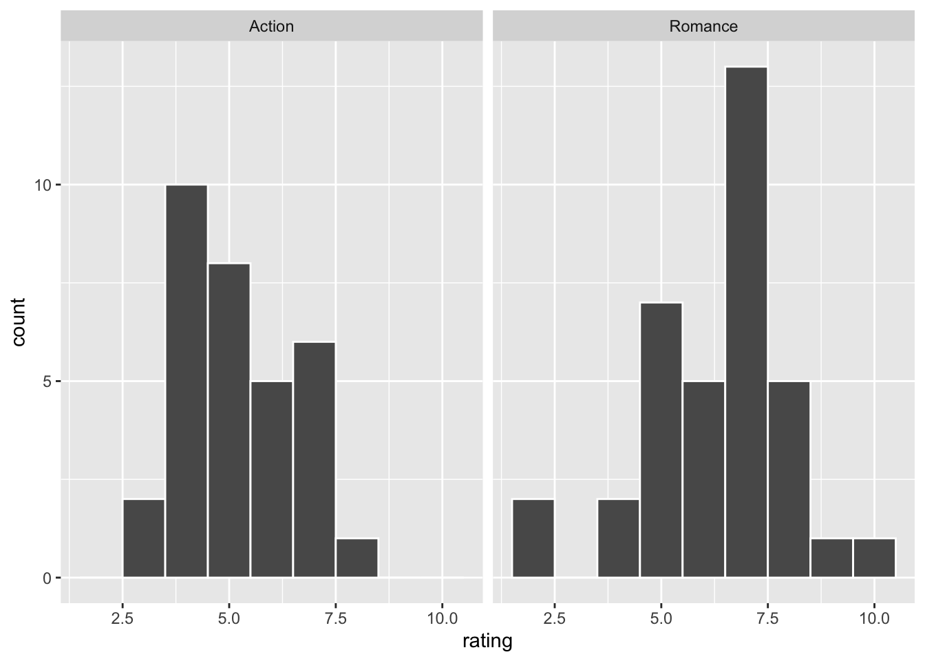
Figure 8.4: Distributions of user ratings for action and romance movies in IMDb.
Both histograms are reasonably close to a bell-shaped normal curve. In addition, the sample sizes for each group are greater than 30, so the assumptions should apply.
Independent samples: The samples should be collected without any natural pairing.
This is met since we sampled the action and romance movies at random and in an unbiased fashion from the database of all IMDb movies.
In summary, we cannot be 100% sure whether all three assumptions have been satisfied. As is often the case in practice, we still proceed with the subsequent test. Should new evidence surface that shows any clear violation of the assumptions, we would need to change the analytical plan.
Two-sample t-statistic
Just as we had to convert the difference in proportions to a \(z\)-statistic by applying Equation (7.2), we need to first standardize the difference of sample mean ratings \(\overline{x}_a - \overline{x}_r\) of action versus romance movies, How? By once again subtracting its mean and dividing by its standard deviation, which gives us the two-sample \(t\)-statistic:
\[ t = \dfrac{ (\bar{x}_a - \bar{x}_r) - (\mu_a - \mu_r)}{ \text{SE}_{\bar{x}_a - \bar{x}_r} } = \dfrac{ (\bar{x}_a - \bar{x}_r) - (\mu_a - \mu_r)}{ \sqrt{\dfrac{{s_a}^2}{n_a} + \dfrac{{s_r}^2}{n_r}} } \tag{8.1} \]
Let’s unpack Equation (8.1) a bit.
In the numerator, \(\bar{x}_a-\bar{x}_r\) is the difference in sample means, while \(\mu_a - \mu_r\) is the difference in population means. In the denominator, \(s_a\) and \(s_r\) are the sample standard deviations of the action and romance movies in our sample movies_sample. Lastly, \(n_a\) and \(n_r\) are the sample sizes of the action and romance movies. Putting this together under the square root gives us the standard error \(\text{SE}_{\bar{x}_a - \bar{x}_r}\).
Observe once again that the formula for \(\text{SE}_{\bar{x}_a - \bar{x}_r}\)
has the sample sizes \(n_a\) and \(n_r\) in them.
So as the sample sizes increase, the standard error goes down.
How can we use the two-sample \(t\)-statistic as a test statistic in our hypothesis test? Assuming the null hypothesis \(H_0: \mu_a - \mu_r = 0\) is true, the right-hand side of the numerator (to the right of the \(-\) sign), \(\mu_a - \mu_r\), becomes 0.
Second, similarly to how the Central Limit Theorem from Chapter 5 states that sample means follow a normal distribution, it can be mathematically proven that the two-sample \(t\)-statistic follows a \(t\)-distribution with degrees of freedom “roughly equal” to \(df = n_a + n_r - 2\). Degrees of freedom can be loosely defined as a measure of how many data points are involved in computing a sample statistic, in this case, the \(t\)-statistic. To better understand this concept of degrees of freedom, we next display three examples of \(t\)-distributions in Figure 8.5 along with the standard normal \(z\) curve.
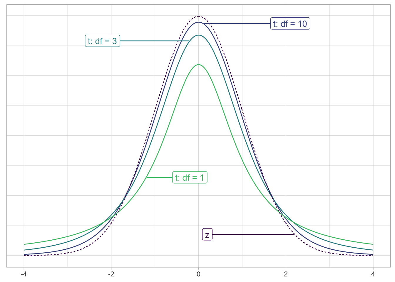
Figure 8.5: Examples of t-distributions and the z curve.
Begin by looking at the center of the plot at 0 on the horizontal axis. As you move up from the value of 0, follow along with the labels and note that the bottom curve corresponds to 1 degree of freedom, the curve above it is for 3 degrees of freedom, the curve above that is for 10 degrees of freedom, and lastly the dotted curve is the standard normal \(z\) curve.
Observe that all four curves have a bell shape, are centered at 0. Compared to the standard normal \(z\)-curve, \(t\)-distributions tend to have more values in the tails of their distributions. As the degrees of freedom increase, or, because the degrees of freedom is tied to the sample size, as sample sizes increase, the \(t\)-distribution more and more resembles the standard normal \(z\) curve. In fact, when the sample size approaches infinity, a \(t\)-distribution becomes a \(z\)-distribution.
The “roughly equal” statement indicates that the equation \(df = n_a + n_r - 2\) is a “good enough” approximation to the true degrees of freedom. The true formula is a bit more complicated than this simple expression, and it does little to build the intuition of the \(t\)-test, so we will not discuss it here.
The message to retain, however, is that small sample sizes lead to small degrees of freedom and thus small sample sizes lead to \(t\)-distributions that are different from the \(z\) curve. In contrast, large sample sizes correspond to large degrees of freedom and thus produce \(t\) distributions that closely align with the standard normal \(z\)-curve.
So, assuming the null hypothesis \(H_0\) is true, our formula for the test statistic simplifies a bit:
\[ t = \dfrac{ (\bar{x}_a - \bar{x}_r) - 0}{ \sqrt{\dfrac{{s_a}^2}{n_a} + \dfrac{{s_r}^2}{n_r}} } = \dfrac{ \bar{x}_a - \bar{x}_r}{ \sqrt{\dfrac{{s_a}^2}{n_a} + \dfrac{{s_r}^2}{n_r}} } \sim t (df = 66) \tag{8.2} \]
where \(df = n_a + n_r -2 = 32 + 36 -2 = 66\)
Observed \(t\)-score
In Section 7.4.1,
we directly calculated the observed \(z\)-score using infer verbs.
We also mentioned an alternative approach:
subtitute each variable in Equation (8.2) with
actual values based on the sample.
Let’s take this approach this time
and compute the values necessary for the observed \(t\)-score.
Recall the summary statistics we computed during our exploratory data analysis
in Section 8.1.1.
movies_sample %>%
  dp$group_by(genre) %>%
  dp$summarize(n = dp$n(), mean_rating = mean(rating), std_dev = sd(rating))
# A tibble: 2 x 4
genre n mean_rating std_dev
* <chr> <int> <dbl> <dbl>
1 Action 32 5.28 1.36
2 Romance 36 6.32 1.61Using these values, the observed two-sample \(t\)-test statistic is
\[ \dfrac{ \bar{x}_a - \bar{x}_r}{ \sqrt{\dfrac{{s_a}^2}{n_a} + \dfrac{{s_r}^2}{n_r}} } = \dfrac{5.28 - 6.32}{ \sqrt{\dfrac{{1.36}^2}{32} + \dfrac{{1.61}^2}{36}} } = -2.906 \tag{8.3} \]
Conducting a \(t\)-test using base-R functions
Now that we have explained behind-the-scenes of a \(t\)-test,
including what test statistic to use and how to compute one,
let’s complete the remaining grunt work with the function t.test()
from the stats package.
Like prop.test() from the stats package in Section 7.4.4,
t.test() also comes with every clean install of R
and requires no extra installation.
stats::t.test(rating ~ genre,
              data = movies_sample,
              alternative = "two.sided",
              conf.level = 1 - ALPHA
)
    Welch Two Sample t-test

data:  rating by genre
t = -2.9059, df = 65.85, p-value = 0.004983
alternative hypothesis: true difference in means is not equal to 0
99.9 percent confidence interval:
 -2.2885491  0.1941046
sample estimates:
 mean in group Action mean in group Romance
             5.275000              6.322222
Note that alternative = "two.sided matches the alternative hypothesis
we defined in Section 8.1.3.
Next, we zoom-in on each line of the output above.
8.1.5 Interpreting output from a t.test()
Line 1-3
Why is the output of t.test() titled “Welch Two sample \(t\)-test?”
[Welch’s \(t\)-test is] an adaptation of Student’s \(t\)-test, and is more reliable when the two samples have unequal variances and/or unequal sample sizes.4
Recall the summary statistics we computed during our exploratory data analysis in Section 8.1.1.
movies_sample %>%
  dp$group_by(genre) %>%
  dp$summarize(n = dp$n(), mean_rating = mean(rating), std_dev = sd(rating))
# A tibble: 2 x 4
genre n mean_rating std_dev
* <chr> <int> <dbl> <dbl>
1 Action 32 5.28 1.36
2 Romance 36 6.32 1.61By default, t.test() uses Welch’s \(t\)-test
unless the two groups have (almost) identical variances and sample sizes.
Line 5
The observed \(t\)-score is -2.906, agreeing with what we have manually computed using Equation (8.3). Also note that the degrees of freedom reported on Line 5, \(df = 65.85\), is slightly different from what we used in Equation (8.2), in which \(df = n_a + n_r -2 = 32 + 36 -2 = 66\). More precisely, degrees of freedom has “shrunken” from 66 to 65.85. This is a direct consequence of applying the Welch’s two-sample \(t\)-test. To “compensate” for the unequal sample sizes and/or variances, the original degree of freedom, 66, took a penalty and got reduced in size, resulting in a slightly more conservative test. The more sample sizes and variances deviate from being equal between two groups, the larger the penalty. The smaller degrees of freedom, 65.85, is also known as the Satterthwaite approximation and involves a quite complicated formula. For most problems, reporting the much simpler \(df = n_1 + n_2 -2\) will suffice.
The \(p\)-value — the probability of observing a \(\lvert t_{66} \rvert\) value of \(\lvert -2.906 \rvert = 2.906\) or more extreme (in both directions) under the null hypothesis — is around 0.005. Given that the \(p\)-value is larger than the pre-determined \(\alpha\) level of 0.001, we fail to reject the null hypotehsis \(H_0: \mu_a - \mu_r = 0\), which leads us to draw the same conclusion as we did using the simulation-based method earlier.
Similar to what we did in Section ??, let’s visualize the \(p\)-value by marking it on the theory-based null-distribution. As usual, we reproduce the simulated-based counterpart from Section 8.1.3 next to it for comparison. Before we do so, can you picture in your mind what they would look like?
# Construct simulation-based null distribution of xbar_a - xbar_r:
null_distribution_movies <- movies_sample %>%
  infer::specify(formula = rating ~ genre) %>%
  infer::hypothesize(null = "independence") %>%
  infer::generate(reps = 1000, type = "permute") %>%
  infer::calculate(stat = "diff in means", order = c("Action", "Romance"))
infer::visualize(null_distribution_movies, bins = 10)
# Construct theory-baseed null distribution of t:
null_distribution_movies_t <- movies_sample %>%
infer::specify(formula = rating ~ genre) %>%
infer::hypothesize(null = "independence") %>%
infer::generate(reps = 1000, type = "permute") %>%
# Notice we switched stat from "diff in means" to "t"
infer::calculate(stat = "t", order = c("Action", "Romance"))
infer::visualize(null_distribution_movies_t, bins = 10)null_dist_1 <- infer::visualize(null_distribution_movies, bins = 10) +
infer::shade_p_value(obs_stat = obs_diff_means,
direction = "both",
fill = c("hotpink"),
size = 1)
null_dist_2 <- infer::visualize(null_distribution_movies_t,
bins = 10,
method = "theoretical") +
infer::shade_p_value(obs_stat = -2.906,
direction = "both",
fill = c("hotpink"),
size = 1)
null_dist_1 + null_dist_2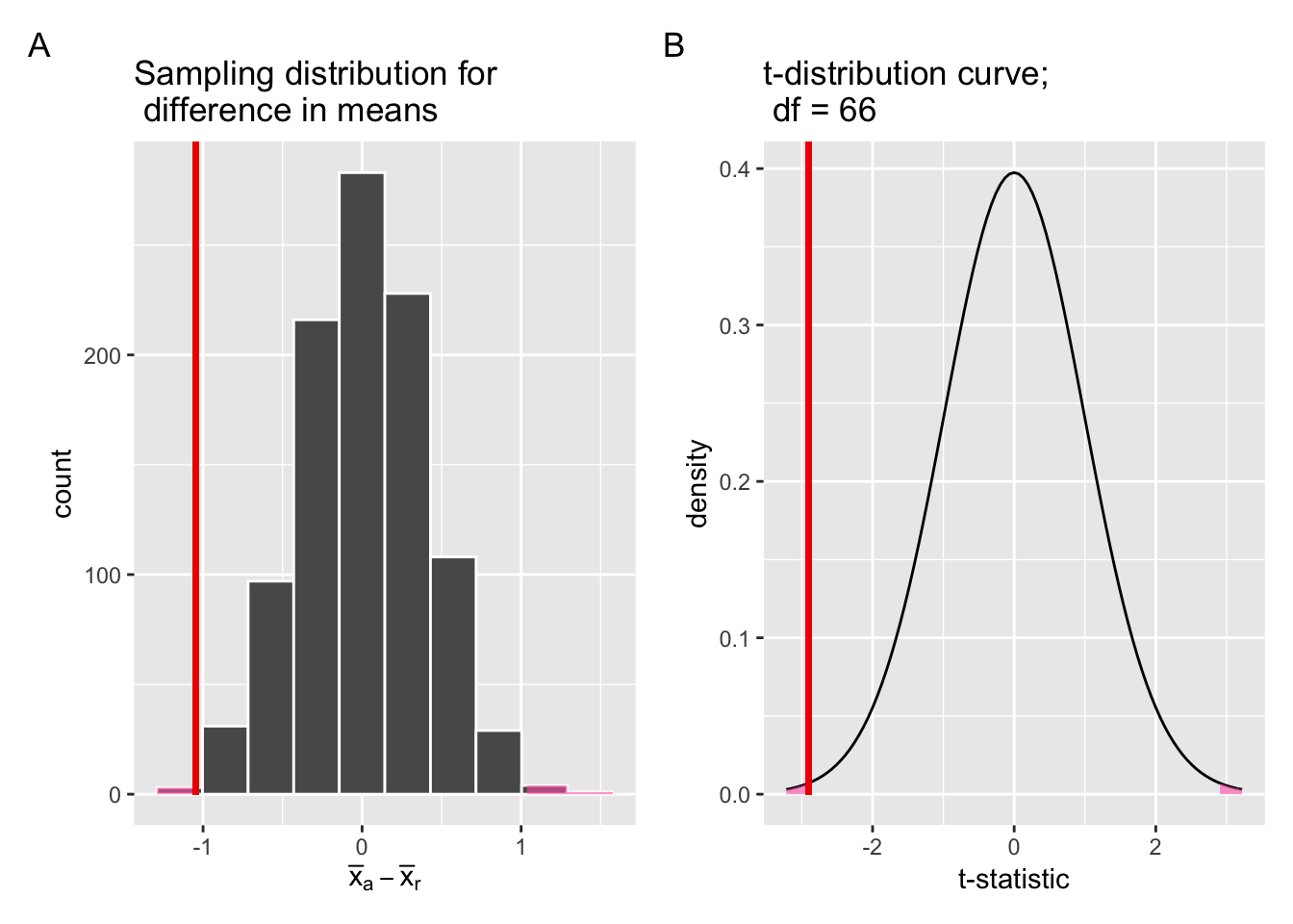
Figure 8.6: Comparing the null distributions of two test statistics.
Similar to Section 7.4.2, the scales on the x-axis between Panel A and B in Figure 8.6 are different, despite the similar shapes of two distributions. In Panel A, each unit on the scale of the x-axis represents one star of actual difference in IMDb ratings between Action and Romance movies. In Panel B, each unit on the scale of the x-axis represents one standard deviation on the \(t\)-distribution curve (\(df\) = 66).
The shaded regions under the \(t\)-distribution curve in Panel B of Figure 8.6 represent the \(p\)-value of the theory-based hypothesis test. Unlike Section 7.4.2, we need to add up the shaded regions on both tails of the distribution, because our alternative hypothesis is a two-sided one: \(H_A: \mu_a - \mu_r \neq 0\).
Line 7-8
t.test() also returned the 99.9% confidence interval of
\(\bar{x}_a - \bar{x}_r\), which is \([-2.29, 0.19]\).
A key value is included in this 99.9% confidence interval for
\(\bar{x}_a - \bar{x}_r\): the value 0.
In other words, at the 99.9% confidence level, or at alpha level
\(\alpha = 0.001\), \(\bar{x}_a\) and \(\bar{x}_r\) are not truly different.
This conclusion corroborates what we found based on \(p\) value previously.
8.1.6 Summary
In this first example, we applied both simulation-based and theory-based methods to the same dataset in order to answer the question: are action or romance movies rated higher. Both methods led to the same conclusion. There is not enough evidence in the current dataset that could support the claim that action and romance movies are rated differently.
8.2 Example 2
Problem statement
Average income varies from one region of the country to another, and it often reflects both lifestyles and regional living expenses. Suppose a new graduate is considering a job in two locations, Cleveland, OH and Sacramento, CA, and he wants to see whether the average income in one of these cities is higher than the other. He would like to conduct a hypothesis test based on two randomly selected samples from the 2000 US Census. (Tweaked a bit from Diez, Barr, and Çetinkaya-Rundel 2014 [Chapter 5])
8.2.1 Competing hypotheses
In words
Null hypothesis: The mean income is the same for both cities.
Alternative hypothesis: The mean income is different for the two cities.
In symbols (with annotations)
- \(H_0: \mu_{sac} = \mu_{cle}\) or \(H_0: \mu_{sac} - \mu_{cle} = 0\), where \(\mu\) represents the average income.
- \(H_A: \mu_{sac} - \mu_{cle} \ne 0\)
8.2.2 Exploring the sample data
cle_sac <- read.delim("https://moderndive.com/data/cleSac.txt") %>%
  dp$rename(
    income = Total_personal_income
  ) %>%
    dp$mutate(
    metro_area = as.factor(Metropolitan_area_Detailed)
        ) %>%
  dp$select(income, metro_area) %>%
  na.omit()
tibble::glimpse(cle_sac)
Rows: 387
Columns: 2
$ income <int> 40240, 13600, 0, 49000, 38300, 14000, 9000, 40000, 18000, …
$ metro_area <fct> Sacramento_ CA, Sacramento_ CA, Sacramento_ CA, Sacramento…# Create a template function for descriptives
my_skim <- skimr::skim_with(base = skimr::sfl(n = length, missing = skimr::n_missing),
numeric = skimr::sfl(
mean,
sd,
iqr = IQR,
min,
p25 = ~ quantile(., 1/4),
median,
p75 = ~ quantile(., 3/4),
max
),
append = FALSE
) #sfl stands for "skimr function list"
cle_sac %>%
dp$group_by(metro_area) %>%
my_skim(income)| Name | Piped data |
| Number of rows | 387 |
| Number of columns | 2 |
| _______________________ | |
| Column type frequency: | |
| numeric | 1 |
| ________________________ | |
| Group variables | metro_area |
Variable type: numeric
| skim_variable | metro_area | n | missing | mean | sd | iqr | min | p25 | median | p75 | max |
|---|---|---|---|---|---|---|---|---|---|---|---|
| income | Cleveland_ OH | 212 | 0 | 27467.07 | 27680.68 | 26800 | 0 | 8475 | 21000 | 35275 | 152400 |
| income | Sacramento_ CA | 175 | 0 | 32427.54 | 35773.63 | 41300 | 0 | 8050 | 20000 | 49350 | 206900 |
The boxplot below also shows the mean for each group highlighted by the red dots.
gg$ggplot(cle_sac, gg$aes(x = metro_area, y = income)) +
  gg$geom_boxplot() +
  gg$stat_summary(fun = "mean", geom = "point", color = "red")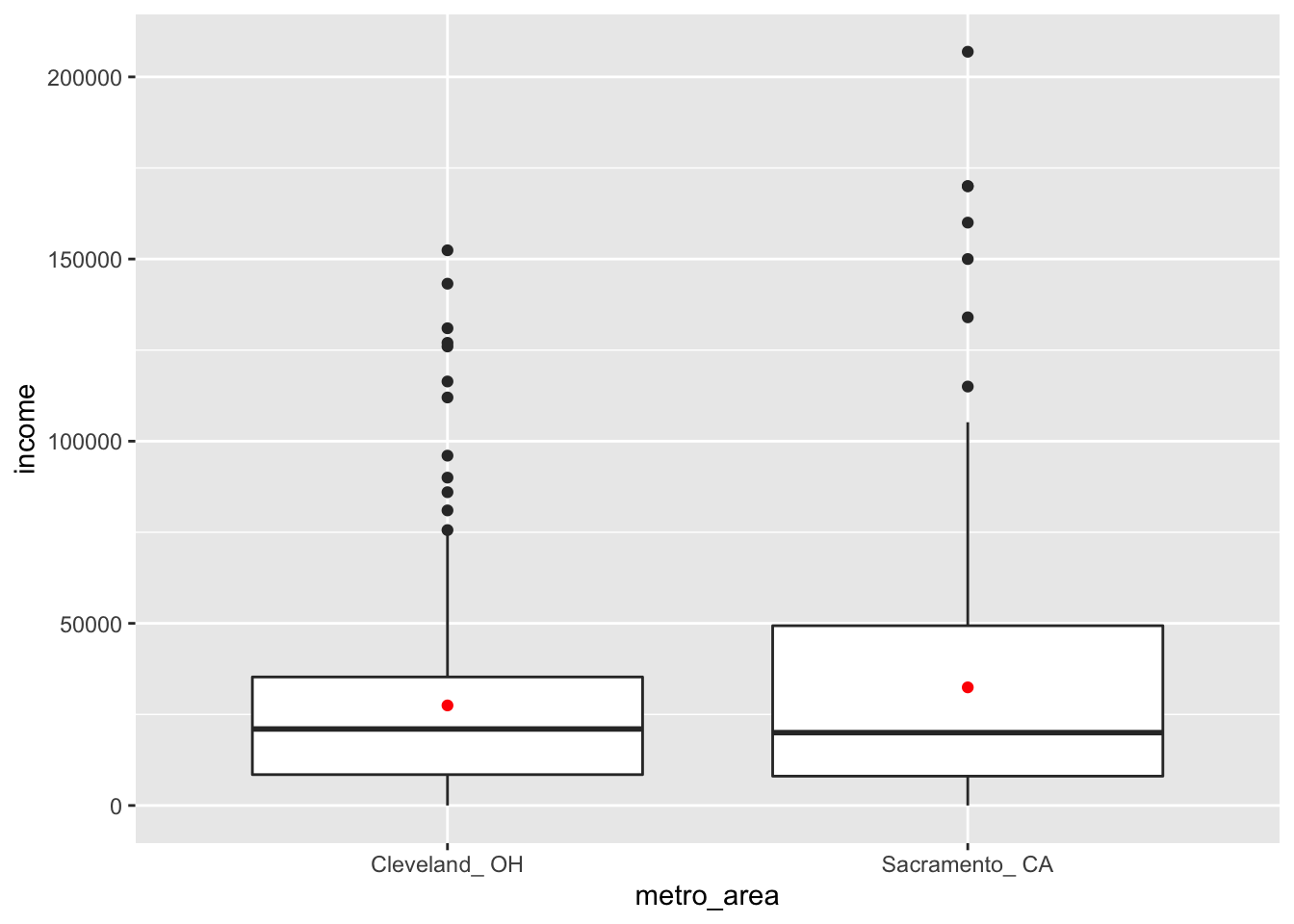
Figure 8.7: Income in two cities
Guess about statistical significance
We are testing whether a difference exists in the mean income of the two levels of the explanatory variable. Based solely on the boxplot, we have reason to believe that no difference exists. The distributions of income seem similar and the means fall in roughly the same place.
8.2.3 Simulation-based methods
Collecting summary info
We now compute the observed statistic:
income_diff <- cle_sac %>%
  infer::specify(income ~ metro_area) %>%
  infer::calculate(
    stat = "diff in means",
    order = c("Sacramento_ CA", "Cleveland_ OH")
  )
income_diff
# A tibble: 1 x 1
stat
<dbl>
1 4960.Hypothesis test using infer verbs
# set random seed for reproducible results
set.seed(2018)
null_distn_two_means <- cle_sac %>%
  infer::specify(income ~ metro_area) %>%
  infer::hypothesize(null = "independence") %>%
  infer::generate(reps = 1000, type = "permute") %>%
  infer::calculate(
    stat = "diff in means",
    order = c("Sacramento_ CA", "Cleveland_ OH")
)infer::visualize(null_distn_two_means) +
infer::shade_p_value(obs_stat = income_diff, direction = "both")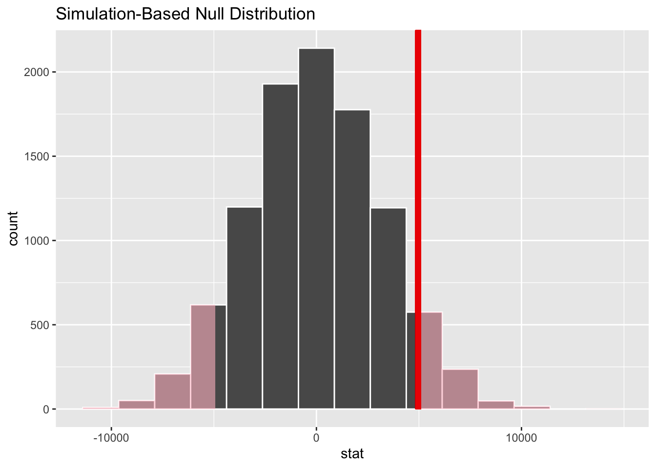
Figure 8.8: Null distribution, observed test statistic, and \(p\)-value.
Recall this is a two-tailed test so we will be looking for values that are greater than or equal to 4960 or less than or equal to -4960 for our \(p\)-value.
Calculate \(p\)-value
pvalue <- null_distn_two_means %>%
  infer::get_pvalue(obs_stat = income_diff, direction = "both")
pvalue
# A tibble: 1 x 1
p_value
<dbl>
1 0.126So our \(p\)-value is 0.126 and we fail to reject the null hypothesis at the 5% level. You can also see this from the histogram above that the observed test statistic are not very far into the tail of the null distribution.
Bootstrapping for confidence interval
We can also create a confidence interval
for the unknown population parameter \(\mu_{sac} - \mu_{cle}\)
using our sample data with bootstrapping.
Here we will bootstrap each of the groups with replacement instead of shuffling.
boot_distn_two_means <- cle_sac %>%
  infer::specify(income ~ metro_area) %>%
  infer::generate(reps = 1000, type="bootstrap") %>%
  infer::calculate(
    stat = "diff in means",
    order = c("Sacramento_ CA", "Cleveland_ OH")
)# A tibble: 1 x 2
lower_ci upper_ci
<dbl> <dbl>
1 -1531. 11516.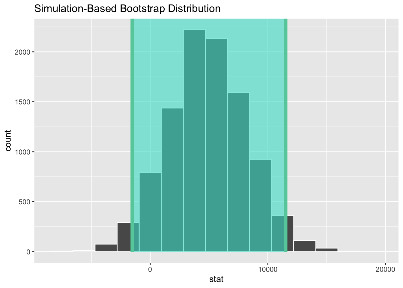
Figure 8.9: Percentile-based 95% confidence interval.
We see that 0 is contained in this confidence interval as a plausible value of \(\mu_{sac} - \mu_{cle}\) (the unknown population parameter). This matches with our hypothesis test results of failing to reject the null hypothesis. Since zero is a plausible value of the population parameter, we do not have enough evidence that Sacramento incomes are different than Cleveland incomes.
Interpretation of the confidence interval: We are 95% confident the true mean yearly income for those living in Sacramento is somewhere between 1531 dollars lower than for Cleveland, to 11516 dollars higher than for Cleveland.
8.2.4 Theory-based method
Check assumptions
Remember that in order to use the short-cut (formula-based, theoretical) approach, we need to check that some assumptions are met.
Independent observations: The observations are independent in both groups.
This condition is met because the cases are randomly selected from each city.
Approximately normal: The distribution of the response for each group should be normal or the sample sizes should be at least 30.
gg$ggplot(cle_sac, gg$aes(x = income)) +
  gg$geom_histogram(color = "white", binwidth = 20000) +
  gg$facet_wrap(~metro_area)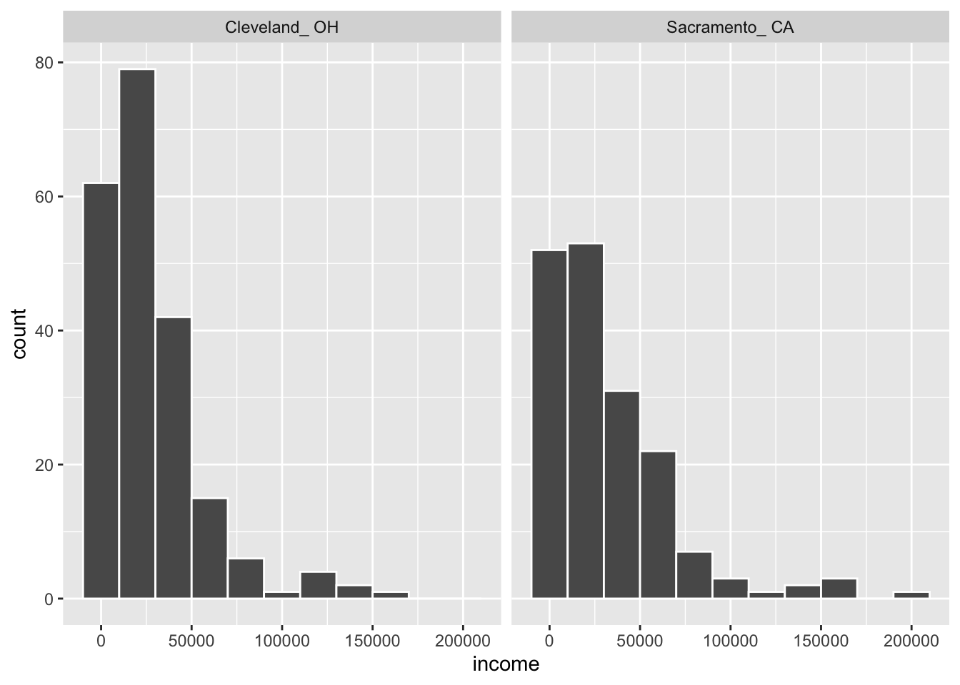
Figure 8.10: Distributions of income in two cities
We have some reason to doubt the normality assumption here because both histograms deviate from a standard normal curve. The sample sizes for each group are greater than 100 though so the assumptions should still apply.
Independent samples: The samples should be collected without any natural pairing.
There is no mention of there being a relationship between those selected in Cleveland and in Sacramento.
Test statistic
Here, we are testing whether the observed difference in sample means (\(\bar{x}_{sac, obs} - \bar{x}_{cle, obs}\) = 4960.48) is statistically different than 0. Assuming that conditions are met and the null hypothesis is true, we can use the \(t\)-distribution to standardize the difference in sample means (\(\bar{x}_{sac} - \bar{x}_{cle}\)) using the approximate standard error of \(\bar{x}_{sac} - \bar{x}_{cle}\) (invoking \(s_{sac}\) and \(s_{cle}\) as estimates of unknown \(\sigma_{sac}\) and \(\sigma_{cle}\)).
\[ t = \frac{ (\bar{x}_{sac} - \bar{x}_{cle}) - (\mu_{sac} - \mu_{cle})}{ \text{SE}_{\bar{x}_{sac} - \bar{x}_{cle}} } = \dfrac{ (\bar{x}_{sac} - \bar{x}_{cle}) - 0}{ \sqrt{\dfrac{{s_{sac}}^2}{n_{sac}} + \dfrac{{s_{cle}}^2}{n_{cle}}} } \sim t (df = n_{sac} + n_{cle} - 2) \tag{8.4} \]
where \(n_{sac} = 175\) for Sacramento and \(n_{cle} = 212\) for Cleveland.
Observed test statistic
    Welch Two Sample t-test

data:  income by metro_area
t = -1.5006, df = 323.36, p-value = 0.1344
alternative hypothesis: true difference in means is not equal to 0
95 percent confidence interval:
 -11463.712   1542.758
sample estimates:
 mean in group Cleveland_ OH mean in group Sacramento_ CA
                    27467.07                     32427.54
We see here that the observed \(t\)-score is around -1.5.
\(p\)-value and confidence interval
The \(p\)-value — the probability of observing a \(\lvert t_{385} \rvert\) value of \(\lvert -1.501 \rvert = 1.501\) or more extreme (in both directions) in our null distribution — is 0.134.
Note that the 95% confidence interval given above matches well with the one calculated using bootstrapping.
State conclusion
We, therefore, do not have sufficient evidence to reject the null hypothesis, \(t\)(385) = -1.5, \(p\) = 0.13. Our initial guess that a statistically significant difference not existing in the means was backed by this statistical analysis. We do not have evidence to suggest that the true mean income differs between Cleveland, OH and Sacramento, CA based on this data (\(\bar{x}_{sac} = 32428\), \(\text{SD}_{sac} = 35774\); \(\bar{x}_{cle} = 27467\), \(\text{SD}_{cle} = 27681\)).5
8.3 Conclusion
So far, we have applied the framework of hypothesis testing
to two types of problems: difference between sample proportions
and difference between sample means.
In each example, both simulation-based method
and theory-based method led to the same conclusion.
Ultimately, it is up to you to decide which method you would choose
for a problem.
However, we believe that the infer framework will prevail
in the long-run for learning.
Learning theory-based methods inevitably
involves memorizing which function to use for which type of test.
In contrast, the infer framework stays more or less the same
for different types of tests.
John Rauser brilliantly elaborated on this point in a 2014
keynote speech:
When I decided to learn statistics, I read several books, which I shall politely not identify. I understood none of them. Most of them simply described statistical procedures and then applied them without any intuitive explanation, or hint at how anyone might have invented these procedures in the first place. And this talk was born of that frustration, and my wish that future students of statistics will learn the deep and elegant ideas at the heart of statistics rather than a confusing grab bag of statistical procedures.
I encourage you to watch the 12-minute keynote speech and appreciate your newly gained understanding of hypothesis testing!
Given that data in both groups deviate from a normal distribution, reporting IQR instead of SD is more appropriate, but SD is more typically reported in the literature. \(\text{IQR}_{sac} = 41300\), \(\text{IQR}_{cle} = 26800\)↩︎