Appendix A Statistical Background
A.1 Basic statistical terms
Note that all the following statistical terms apply only to numerical variables, except the distribution which can exist for both numerical and categorical variables.
A.1.1 Mean
The mean is the most commonly reported measure of center.
It is commonly called the average though this term can be a little ambiguous.
The mean is the sum of all of the data elements
divided by how many elements there are.
If we have \(n\) data points, the mean is given by:
\[ Mean = \frac{x_1 + x_2 + \cdots + x_n}{n} \tag{5.1} \]
A.1.2 Median
The median is calculated by first sorting a variable’s data from smallest to largest. After sorting the data, the middle element in the list is the median. If the middle falls between two values, then the median is the mean of those two middle values.
A.1.3 Standard deviation
We will next discuss the standard deviation (\(sd\)) of a variable.
The formula can be a little intimidating at first
but it is important to remember that it is essentially a measure
of how far we expect a given data value will be from its mean:
\[ sd = \sqrt{\frac{(x_1 - Mean)^2 + (x_2 - Mean)^2 + \cdots + (x_n - Mean)^2}{n - 1}} \tag{5.2} \]
A.1.4 Five-number summary
The five-number summary consists of five summary statistics: the minimum, the first quantile AKA 25th percentile, the second quantile AKA median or 50th percentile, the third quantile AKA 75th, and the maximum. The five-number summary of a variable is used when constructing boxplots, as seen in Section 2.7.
The quantiles are calculated as
- first quantile (\(Q_1\)): the median of the first half of the sorted data
- third quantile (\(Q_3\)): the median of the second half of the sorted data
The interquartile range (IQR) is defined as \(Q_3 - Q_1\) and is a measure of how spread out the middle 50% of values are. The IQR corresponds to the length of the box in a boxplot.
The median and the IQR are not influenced by the presence of outliers in the ways that the mean and standard deviation are. They are, thus, recommended for skewed datasets. We say in this case that the median and IQR are more robust to outliers.
A.2 Populations and samples
You may have seen both concepts — population and sample — in various contexts.
“Scientists estimate the monarch population in the eastern U.S. and southern Canada has fallen about 80 per cent since the mid-1990s.”
“City starts collecting wastewater samples for COVID-19 testing”
In the world of statistics, these two concepts exist mostly because we want to answer research questions like the following:
Is Universal Health Care a protective factor against cancer mortality?
https://www.sciencedirect.com/science/article/abs/pii/S0140673616005778
Is discrimination responsible for the gender wage gap?
Will the made-in-Canada covid vaccine be effective?
https://www.cbc.ca/news/health/covid-19-vaccine-providence-1.5887613
What is the average time to complete a Master’s degree at Carleton?
Quite often, it is impractical to study every case in a population, either bacause doing so would take too long, or cost too much. Instead, a sample is collected.
Sample is both a noun — a sample, and a verb — to sample, sampling.
A.2.1 Distribution
Where there is sampling, there is a distribution that describes
how frequently different values of a variable in the sample occur.
Looking at the visualization of a distribution
can show where the values are centered, show how the values vary,
and give some information about where a typical value might fall.
Recall from Chapter 2 that we can visualize the distribution of a numerical variable using binning in a histogram and that we can visualize the distribution of a categorical variable using a barplot.
Consider the “average program length” example. Instead of polling every student who have ever graduated from a Master’s program at Carleton, which would be a huge undertaking, we sampled 100 alumni, and obtained the following data.
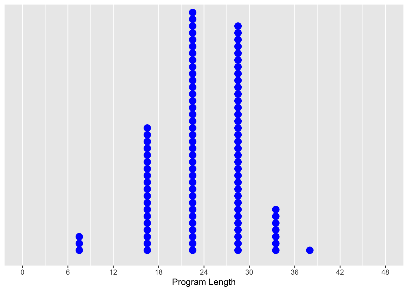
Figure A.1: 100 alumni and length of their Master’s program.
This reminds us of …
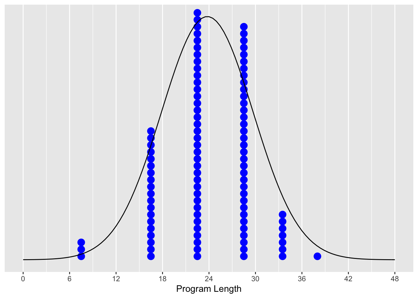
Figure A.2: A bell curve.
A.2.2 Normal distribution
Normal distributions are a family of distributions with a symmetrical bell shape. It was first described by De Moivre in 1733 and subsequently by the German mathematician C. F. Gauss (1777 - 1885). Informally called a bell curve, although many other distributions are also bell-shaped, including t-distirbutions.
All normal distributions are defined by two values: (1) the mean \(\mu\) (“mu”) which locates the center of the distribution and (2) the standard deviation \(\sigma\) (“sigma”) which determines the variation of the distribution. This is also evidenced in Equation (A.1). Despite its sophisticated look, it only contains two unknowns — \(\mu\) and \(\sigma\), with the rest all being constants (i.e., \(e\), \(\pi\)).
\[ f(x) = \frac{1}{{\sigma \sqrt {2\pi } }}e^{{ - \frac{1}{2} {\left( \frac{x - \mu} {\sigma} \right)}^2 }} \tag{A.1} \]
In Figure A.3, we plot three normal distributions where:
- The solid normal curve has mean \(\mu = 5\) & standard deviation \(\sigma = 2\).
- The dotted normal curve has mean \(\mu = 5\) & standard deviation \(\sigma = 5\).
- The dashed normal curve has mean \(\mu = 15\) & standard deviation \(\sigma = 2\).
Normal distribution is the umbrella term for a family of distributions, all feature the same bell curve and the underlying density function.
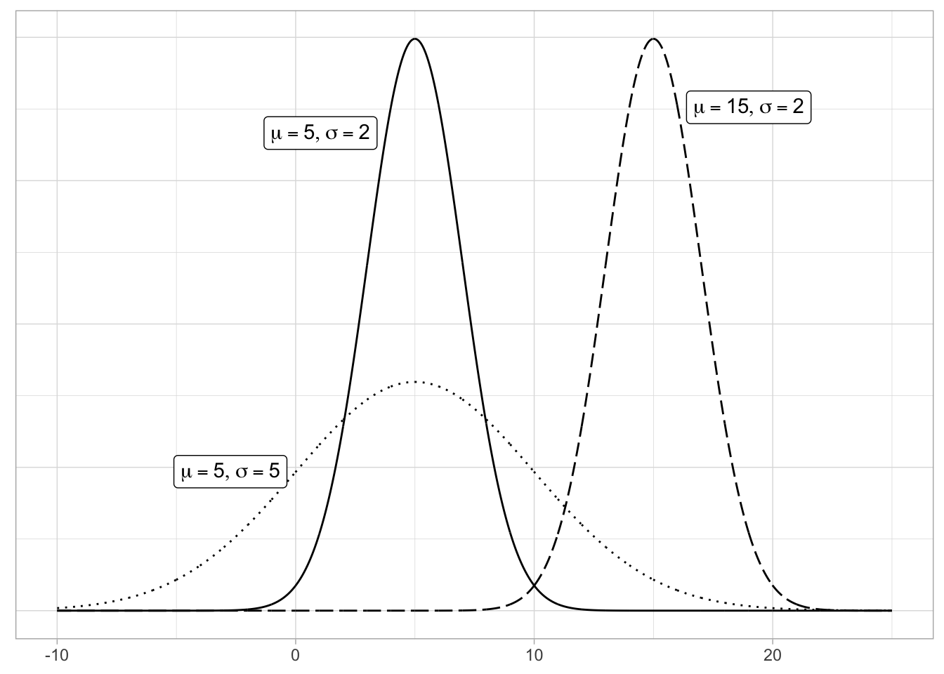
Figure A.3: Three nromal distributions.
Notice how the solid and dotted line normal curves have the same center due to their common mean \(\mu\) = 5. However, the dotted line normal curve is wider due to its larger standard deviation of \(\sigma\) = 5. On the other hand, the solid and dashed line normal curves have the same variation due to their common standard deviation \(\sigma\) = 2. However, they are centered at different locations. Area under every curve is invariably 1.
The simplest case is known as the standard normal distirbution, where \(\mu\) is 0 and \(\sigma\) is 1.
Furthermore, if a variable follows a normal curve, there is a rule of thumb we can use:
95% of values will lie within \(\pm\) 1.96 \(\approx\) 2 standard deviations of the mean.
Let’s illustrate this on a standard normal curve in Figure A.4. The dashed lines are at -1.96 and 1.96. The areas under the normal curve add up to 100%. For example:
- The middle segment represent the interval \(-1.96\) to \(1.96\). The shaded area between this interval represents 95% of the area under the curve. In other words, 95% of values in this distirbution are between 2 standard deviations below and above the mean, give or take.
- The two tails represent the interval \(-\infty\) to \(-1.96\), and \(1.96\) to \(\infty\), respectively. Each tail represents 2.5% of the area under the curve, or two tails combined represent 5% of the area under the curve. In other words, a total of 5% of values in this distribution are either 2 standard deviations larger or smaller than the average.
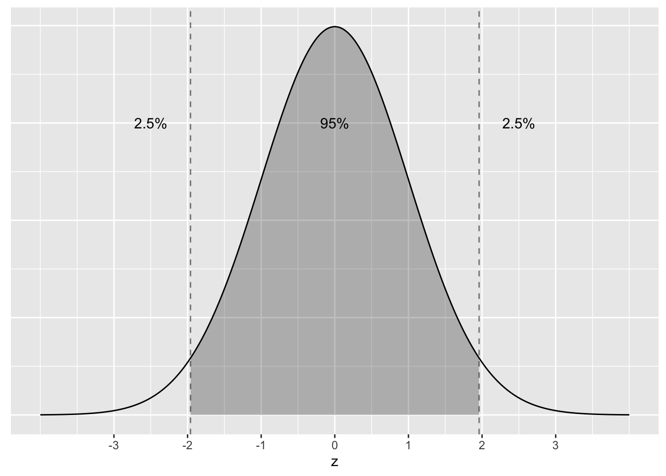
Figure A.4: Rules of thumb about areas under normal curves.
In statistics, the standard normal distribution is the most important continuous probability distribution, largely because of what’s known as the central limit theorem.