Appendix B Inference Examples
This appendix is designed to provide you with examples of basic hypothesis tests and their corresponding confidence intervals. Traditional theory-based methods as well as computational-based methods are presented.
Needed packages
# Install xfun so that I can use xfun::pkg_load2
if (!requireNamespace('xfun')) install.packages('xfun')
xf <- loadNamespace('xfun')

cran_packages <- c(
                  "dplyr",
                  "ggplot2",
                  "infer"
)

if (length(cran_packages) != 0) xf$pkg_load2(cran_packages)

gg <- import::from(ggplot2, .all=TRUE, .into={new.env()})
dp <- import::from(dplyr, .all=TRUE, .into={new.env()})

import::from(magrittr, "%>%")
import::from(patchwork, .all=TRUE)
B.1 One mean
B.1.1 Problem statement
The National Survey of Family Growth conducted by the Centers for Disease Control gathers information on family life, marriage and divorce, pregnancy, infertility, use of contraception, and men’s and women’s health. One of the variables collected on this survey is the age at first marriage. 5,534 randomly sampled US women between 2006 and 2010 completed the survey. The women sampled here had been married at least once. Do we have evidence that the mean age of first marriage for all US women from 2006 to 2010 is greater than 23 years? (Tweaked a bit from Diez, Barr, and Çetinkaya-Rundel 2014 [Chapter 4])
B.1.2 Competing hypotheses
In words
Null hypothesis: The mean age of first marriage for all US women from 2006 to 2010 is equal to 23 years.
Alternative hypothesis: The mean age of first marriage for all US women from 2006 to 2010 is greater than 23 years.
In symbols (with annotations)
\(H_0: \mu = \mu_{0}\), where \(\mu\) represents the mean age of first marriage for all US women from 2006 to 2010 and \(\mu_0\) is 23.
\(H_A: \mu > 23\)
Set \(\alpha\)
It’s important to set the significance level before starting the testing using the data. Let’s set the significance level at 5% here.
B.1.3 Exploring the sample data
# Create a template function for descriptives to be recycled
my_skim <- skimr::skim_with(base = skimr::sfl(n = length, missing = skimr::n_missing),
                     numeric = skimr::sfl(
                                          mean,
                                          sd,
                                          iqr = IQR,
                                          min,
                                          p25 = ~ quantile(., 1/4),
                                          median,
                                          p75 = ~ quantile(., 3/4),
                                          max
                                          ),
                            append = FALSE
) #sfl stands for "skimr function list"| Name | Piped data |
| Number of rows | 5534 |
| Number of columns | 1 |
| _______________________ | |
| Column type frequency: | |
| numeric | 1 |
| ________________________ | |
| Group variables | None |
Variable type: numeric
| skim_variable | n | missing | mean | sd | iqr | min | p25 | median | p75 | max |
|---|---|---|---|---|---|---|---|---|---|---|
| age | 5534 | 0 | 23.44 | 4.72 | 6 | 10 | 20 | 23 | 26 | 43 |
The histogram below also shows the distribution of age.
gg$ggplot(data = age_at_marriage, mapping = gg$aes(x = age)) +
  gg$geom_histogram(binwidth = 3, color = "white")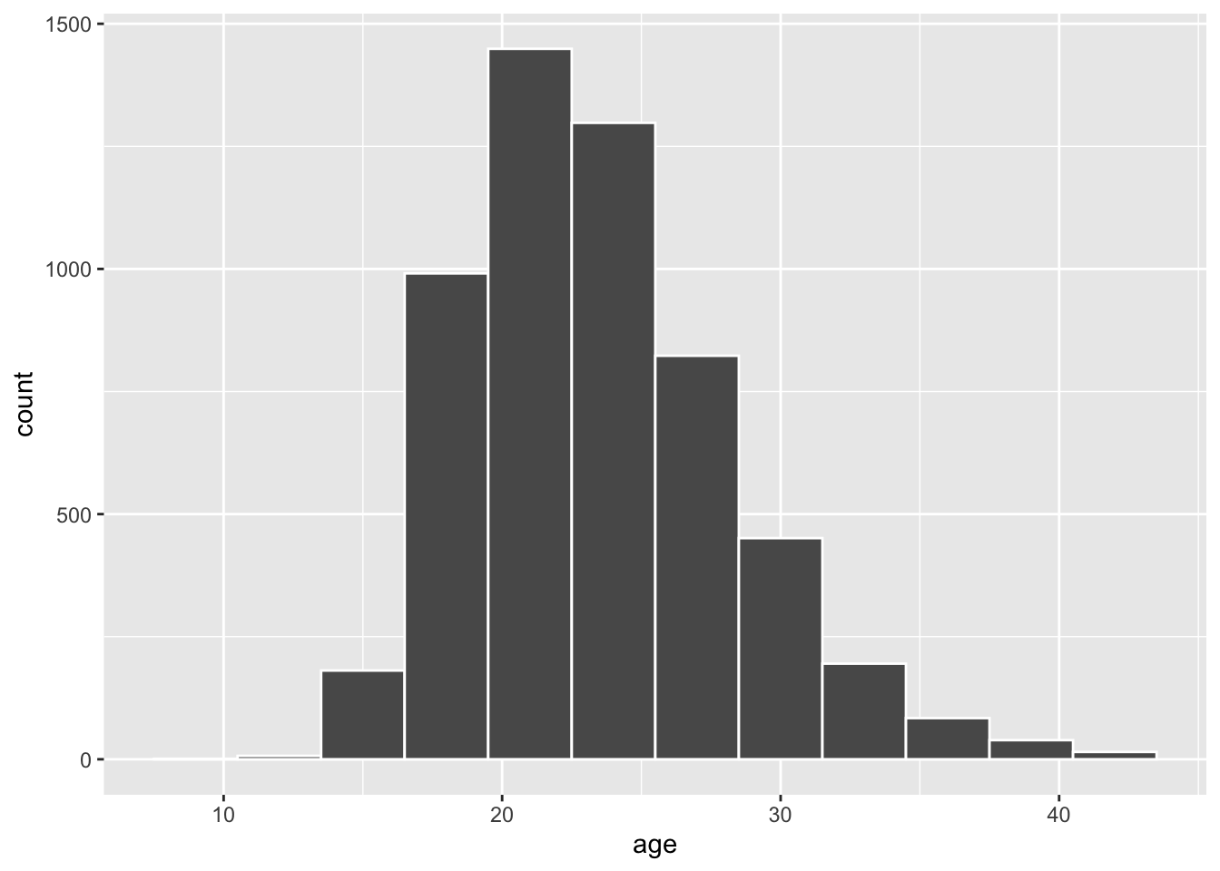
Figure B.1: Distribution of age at first marriage for women in US between 2006-2010.
The observed statistic of interest here is the sample mean:
x_bar <- age_at_marriage %>%
  infer::specify(response = age) %>%
  infer::calculate(stat = "mean")
x_bar
# A tibble: 1 x 1
stat
<dbl>
1 23.4Note that the code above to calculate x_bar is equivalent to the following:
Guess about statistical significance
We are testing whether the observed sample mean of 23.44 is statistically greater than \(\mu_0 = 23\). They seem to be quite close, but we have a large sample size here. I am going to guess that the large sample size will lead us to reject this practically trivial difference.
B.1.4 Simulation-based methods
Bootstrapping for hypothesis test
To find out whether the observed sample mean of 23.44 is statistically greater than \(\mu_0 = 23\), we need to account for the sample size. We also need to determine a process that replicates how the original sample (\(n = 5534\)) was selected.
We can use the idea of bootstrapping to simulate the population from which the sample came and then generate samples from that simulated population to account for sampling variability.
set.seed(2018)
null_distn_one_mean <- age_at_marriage %>%
  infer::specify(response = age) %>%
  # `null = point` because the hypothesis only involves a single sample
  infer::hypothesize(null = "point", mu = 23) %>%
  infer::generate(reps = 1000) %>%
  infer::calculate(stat = "mean")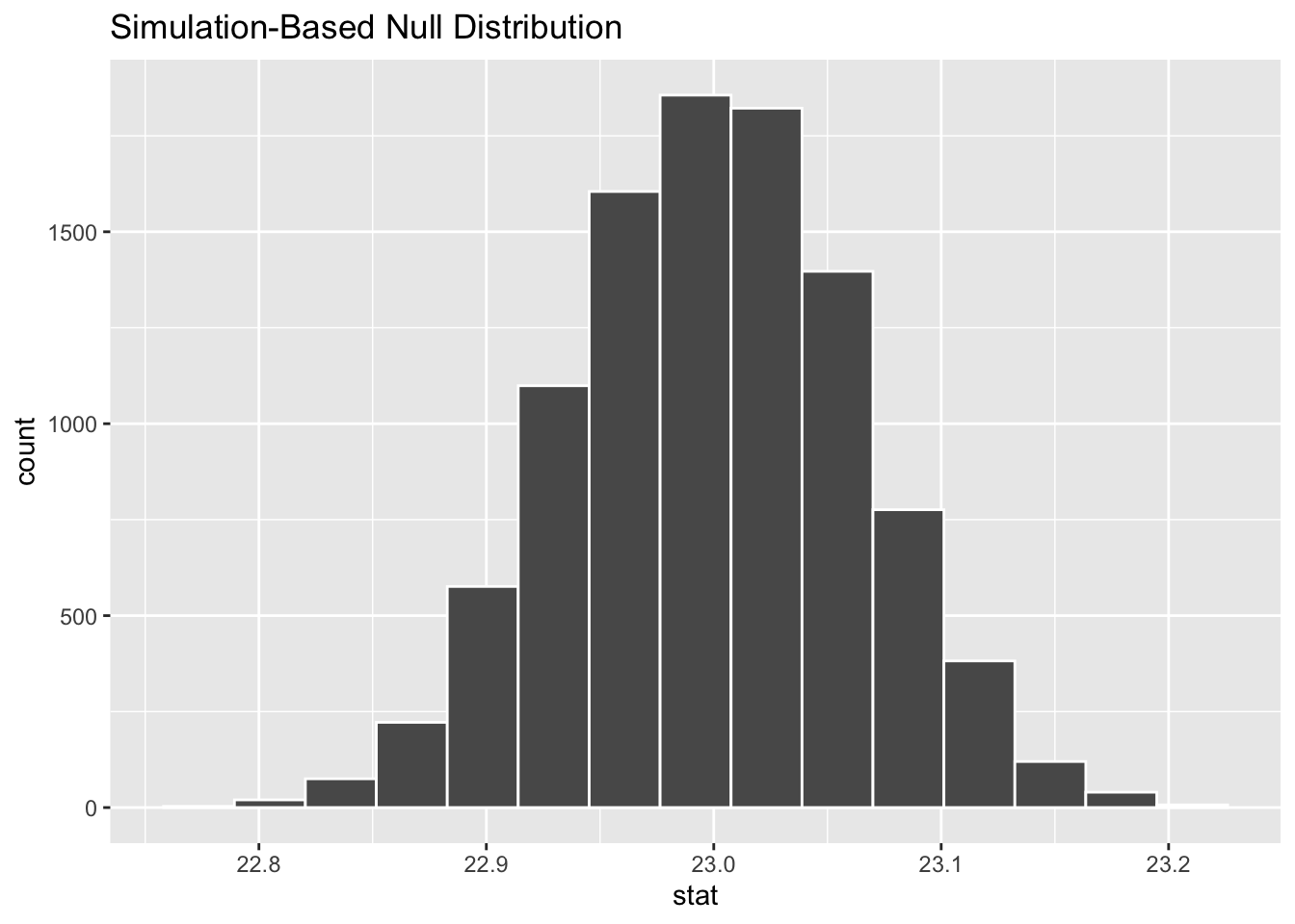
Figure B.2: Null distribution for age using bootstrapping.
Good to know
How was the sampling distribution in Figure B.2 created?
Sample with replacement from the original sample of 5534 women and repeat this process 1,000 times,
calculate the mean for each of the 1,000 bootstrap samples created in Step 1.,
combine all of these bootstrap statistics calculated in Step 2 into a
boot_distnobject, andshift the center of this distribution over to the null value of 23. (This is needed; otherwise it will be centered at 23.44 as a result of the bootstrapping process)
Next, we can use this distribution to observe our \(p\)-value. Recall this is a right-tailed test so we will be looking for values that are greater than or equal to 23.44 for our \(p\)-value.
infer::visualize(null_distn_one_mean) +
  infer::shade_p_value(obs_stat = x_bar, direction = "greater")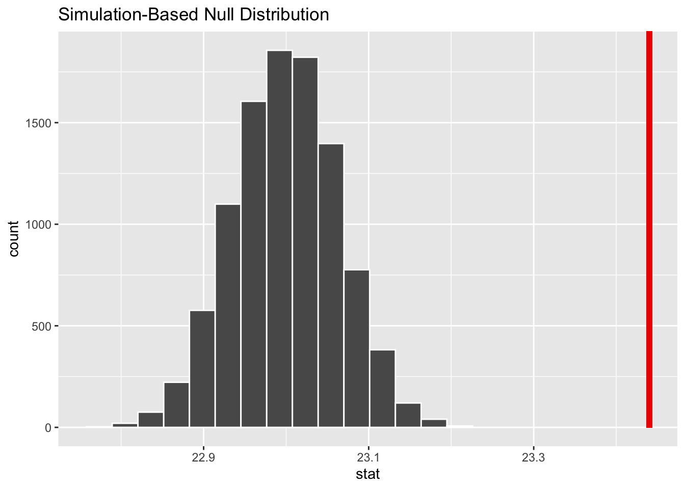
Figure B.3: Null distribution for age using bootstrapping; red vertical line = observed test statistic.
When you run the chunk above, you will likely have received a warning which reads:
Warning message: Please be cautious in reporting a p-value of 0. This result is an approximation based on the number of
repschosen in thegenerate()step. See?get_p_value()for more information.
Be definition, a \(p\)-value could be infinitely small, but never be zero.
However, the output of infer::get_p_value() could be zero,
if none of the test statistic from the infer::calculate() step
is equal or larger than the observed statistic.
This is largely an artifical effect.
In the case that a \(p\)-value of zero is returned
by infer::get_p_value(),
the true size of \(p\)-value is likely smaller than 3/reps.
For example, if reps = 3000,
and if infer::get_p_value() returns a 0,
then you can report p < 0.001.
So the current \(p\)-value led us to reject the null hypothesis at the 5% level. You can also see this from the histogram above that we are far into the tail of the null distribution.
Bootstrapping for confidence interval
We can also create a confidence interval for the unknown population parameter \(\mu\) using our sample data using bootstrapping.
boot_distn_one_mean <- age_at_marriage %>%
  infer::specify(response = age) %>%
  infer::generate(reps = 1000) %>%
infer::calculate(stat = "mean")# A tibble: 1 x 2
lower_ci upper_ci
<dbl> <dbl>
1 23.3 23.6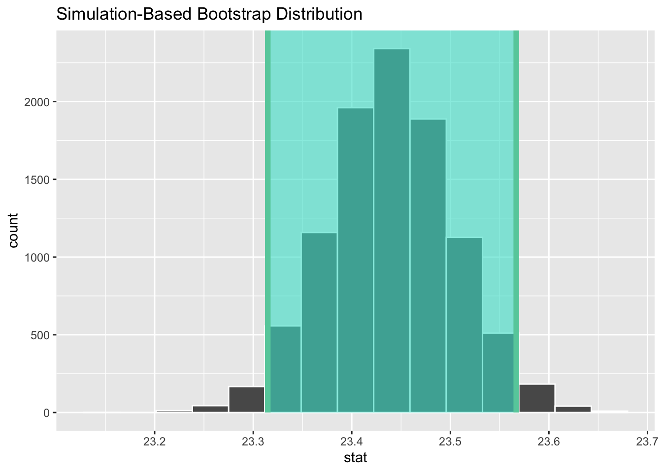
Figure B.4: A 95% confidence interval for the mean age of US women who get married between 2006 to 2010.
Note that although the alternative hypothesis \(H_A\) is one-sided in the current example, a confidence interval is typically closed on both sides, i.e., a two-sided one, as shown above.
We see that \(\mu_0 = 23\) is not contained in this confidence interval as a plausible value of \(\mu\) (the unknown population mean) and the entire interval is larger than 23. This matches with our hypothesis test results of rejecting the null hypothesis in favor of the alternative (\(\mu > 23\)).
Interpretation: We are 95% confident that the true mean age of first marriage for all US women from 2006 to 2010 is between 23.31 and 23.57.
B.1.5 Theory-based methods
Check conditions
Remember that in order to use the shortcut (formula-based, theoretical) approach, we need to check that some conditions are met.
Independent observations: The observations are collected independently.
The cases are selected independently through random sampling so this condition is met.
Approximately normal: The distribution of the response variable should be normal or the sample size should be at least 30.
The histogram for the sample above does show some skewness (Figure B.1).
The Q-Q plot below also shows some skewness.
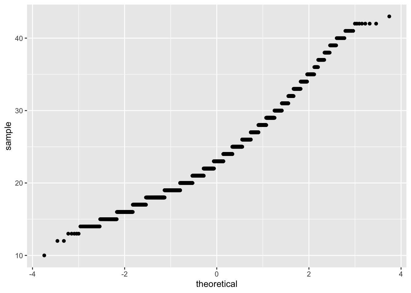
Figure B.5: Q-Q plot for age.
The sample size here is quite large though (\(n = 5534\)) so both conditions are met.
Good to know
How to read a Q-Q plot?
Q-Q stands for quantile-quantile. When we apply a Q-Q plot to a sample of data, for example, it can tell us whether the data follow a normal distribution or not. If the data do follow a normal distribution, we should observe a straight line formed by points extending to both upper right corner and bottom left corner.
Like a histogram, a Q-Q plot is a visual check, not a rigorous proof, so it is somewhat subjective. A straight line with some small deviation can still be accepted as normally distributed.
Test statistic
Our target unknown parameter is the population mean \(\mu\). A good guess of it is the sample mean \(\bar{x}\). Recall that this sample mean is actually a random variable that will vary as different samples are (theoretically, would be) collected. We are testing how likely it is for us to have observed a sample mean of \(\bar{x}_{obs} = 23.44\) or larger assuming that the population mean is 23 (i.e., under the null hypothesis). If the conditions are met and assuming \(H_0\) is true, we can “standardize” this original test statistic of \(\bar{x}\) into a \(t\)-statistic that follows a \(t\)-distribution with degrees of freedom equal to \(df = n - 1\):
\[ t =\dfrac{ \bar{x} - \mu_0}{ s / \sqrt{n} } \sim t (df = n - 1) \]
where \(s\) represents the standard deviation of the sample and \(n\) is the sample size.
Observed test statistic
While one could compute this observed test statistic by “hand,”
the focus here is on the set-up of the problem
and in understanding which formula for the test statistic applies.
We can use the t_test() function to perform this analysis for us.
    One Sample t-test

data:  age_at_marriage$age
t = 6.9357, df = 5533, p-value = 0.000000000002252
alternative hypothesis: true mean is greater than 23
95 percent confidence interval:
 23.33578      Inf
sample estimates:
mean of x
 23.44019
We see here that the \(t_{obs}\) value is 6.94.
Compute \(p\)-value
The \(p\)-value—the probability of observing an \(t_{obs}\) value
of 6.94 or more in our null distribution
of a \(t\) with 5533 degrees of freedom—
is smaller than 0.001.
State conclusion
We, therefore, have sufficient evidence to reject the null hypothesis, \(t(1) = 6.94\), \(p < 0.001\). Our initial guess that our observed sample mean was statistically greater than the hypothesized mean has supporting evidence here. Based on this sample, we have evidence that the mean age of first marriage for all US women from 2006 to 2010 is greater than 23 years, (\(M = 23.44\)).
Confidence interval
Note on line 7-8 of the output from the previous t.test(),
the 95% confidence interval has Inf as its upperbound.
This is because the \(t\)-test we conducted was one-sided.
As mentioned earlier, a confidence interval is typically two-sided.
Simimlar to the two-sided confidence interval we constructed using bootstrapping,
let’s request a theory-based two-sided confidence interval using t.test().
[1] 23.31577 23.56461
attr(,"conf.level")
[1] 0.95
B.1.6 Comparing results
Observing the bootstrap distribution in Section B.1.4, it makes sense that the results are so similar for theory-based and simulation-based methods in terms of the \(p\)-value and the confidence interval, because these distributions look very similar to normal distributions. Give that the conditions for the theory-based method were met (the large sample size was the driver here), we could make an educated guess that using either method will lead to similar results.
B.2 Two means (paired samples)
Problem statement
Trace metals in drinking water affect the flavor and an unusually high concentration can pose a health hazard. Ten pairs of data were taken measuring zinc concentration in bottom water and surface water at 10 randomly selected locations on a stretch of river. Do the data suggest that the true average concentration in the surface water is smaller than that of bottom water? (Note that units are not given.) [Tweaked a bit from https://onlinecourses.science.psu.edu/stat500/node/51]
B.2.1 Competing hypotheses
In words
Null hypothesis: The mean concentration in the bottom water is the same as that of the surface water at different paired locations.
Alternative hypothesis: The mean concentration in the surface water is smaller than that of the bottom water at different paired locations.
In symbols (with annotations)
\(H_0: \mu_{diff} = 0\), where \(\mu_{diff}\) represents the mean difference in concentration for surface water minus bottom water.
\(H_A: \mu_{diff} < 0\)
Set \(\alpha\)
It’s important to set the significance level before starting the testing using the data. Let’s set the significance level at 5% here.
B.2.2 Exploring the sample data
# A tibble: 6 x 3
  loc_id location concentration
   <dbl> <chr>            <dbl>
1      1 bottom           0.43
2      1 surface          0.415
3      2 bottom           0.266
4      2 surface          0.238
5      3 bottom           0.567
6      3 surface          0.39
Let’s compute the differences in surface - bottom for each of the 10 locations
and save it in a new column pair_diff.
zinc_diff <- zinc_tidy %>%
  dp$group_by(loc_id) %>%
  dp$summarize(pair_diff = diff(concentration)) %>%
  dp$ungroup()
zinc_diff
# A tibble: 10 x 2
loc_id pair_diff
* <dbl> <dbl>
1 1 -0.015
2 2 -0.028
3 3 -0.177
4 4 -0.121
5 5 -0.102
6 6 -0.107
7 7 -0.019
8 8 -0.0660
9 9 -0.0580
10 10 -0.111 Good to know
Paired data
Even though the current research question appears to involve two groups of data:
zinc concentration in the surface water,
and zinc concentration in the bottom water,
it is the difference between each pair that we are interested in,
that is, the 10 numbers in the newly derived data frame zinc_diff.
More precisely, we are asking whether the true difference of zinc concentration
in the population, represented by a sample of 10 in zinc_diff,
is zero or not.
This can be further reframed as: is the average of those 10 values in zinc_diff
meaningfully (statistically) different from zero?
Recall that in the previous example,
we asked the question whether the average age of wommen at their first marriage
was different from 23.
These two questions in essence are of the same type,
barring differences in specific names and values.
Therefore we can apply the same method we had seen in the previous example
to the current one.
Testing the difference between paired data is a common type of research question. These paired data can arise from research scenarios such as:
A group of 20 patients received a therapy. Each patient was measured twice on their symptoms, before and after the therapy, to assess the effectiveness of the therapy. The paired data consist of measurements taken at two different times for each patient — pre- and post-therapy.
A company doing market research hired a group of 10 wine connoisseurs (a.k.a, oenophiles) to taste two types of wine. Each wine taster gave two ratings, one for each type of wine. The paired data consist of ratings for two types of wine from each wine taster. The researchers could calculate the differences beteeween each pair of ratings and test whether the two types of wine are truely different.
All of these scenarios share one common feature: there are always two samples in which observations in one sample can be paired with observations in othe other sample. For this reason, the theory-based method applied to those data is commonly known as a paired \(t\)-test.
Next we calculate the mean difference as our observed statistic:
d_hat <- zinc_diff %>%
  infer::specify(response = pair_diff) %>%
  infer::calculate(stat = "mean")
d_hat
# A tibble: 1 x 1
stat
<dbl>
1 -0.0804The histogram below also shows the distribution of pair_diff.
gg$ggplot(zinc_diff, gg$aes(x = pair_diff)) +
  gg$geom_histogram(binwidth = 0.04, color = "white") +
  gg$labs(x = "Zinc concentration in the surface water minus bottom water")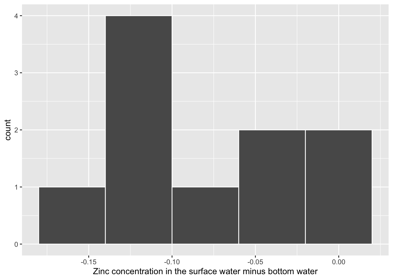
Figure B.6: Distribution of zinc concentration difference at a sample of 10 locations.
Guess about statistical significance
We are testing whether \(\hat{x}_{diff}\), or the sample paired mean difference of -0.0804, is statistically less than 0. They seem to be quite close, and we have a small number of pairs (\(n = 10\)). Let’s guess that we will fail to reject the null hypothesis.
B.2.3 Simulation-based methods
Bootstrapping for hypothesis test
To find out whether the observed sample mean difference \(\bar{x}_{diff} = -0.0804\) is statistically less than 0, we need to account for the number of pairs. Treating the differences as our data of interest, we can build bootstrap samples similar to how we did in the one sample mean example. We hypothesize that the mean difference is zero.
set.seed(2018)
null_distn_paired_means <- zinc_diff %>%
  infer::specify(response = pair_diff) %>%
  infer::hypothesize(null = "point", mu = 0) %>%
  infer::generate(reps = 1000) %>%
infer::calculate(stat = "mean")infer::visualize(null_distn_paired_means) +
gg$labs(x = "Paired mean difference of zinc concentration")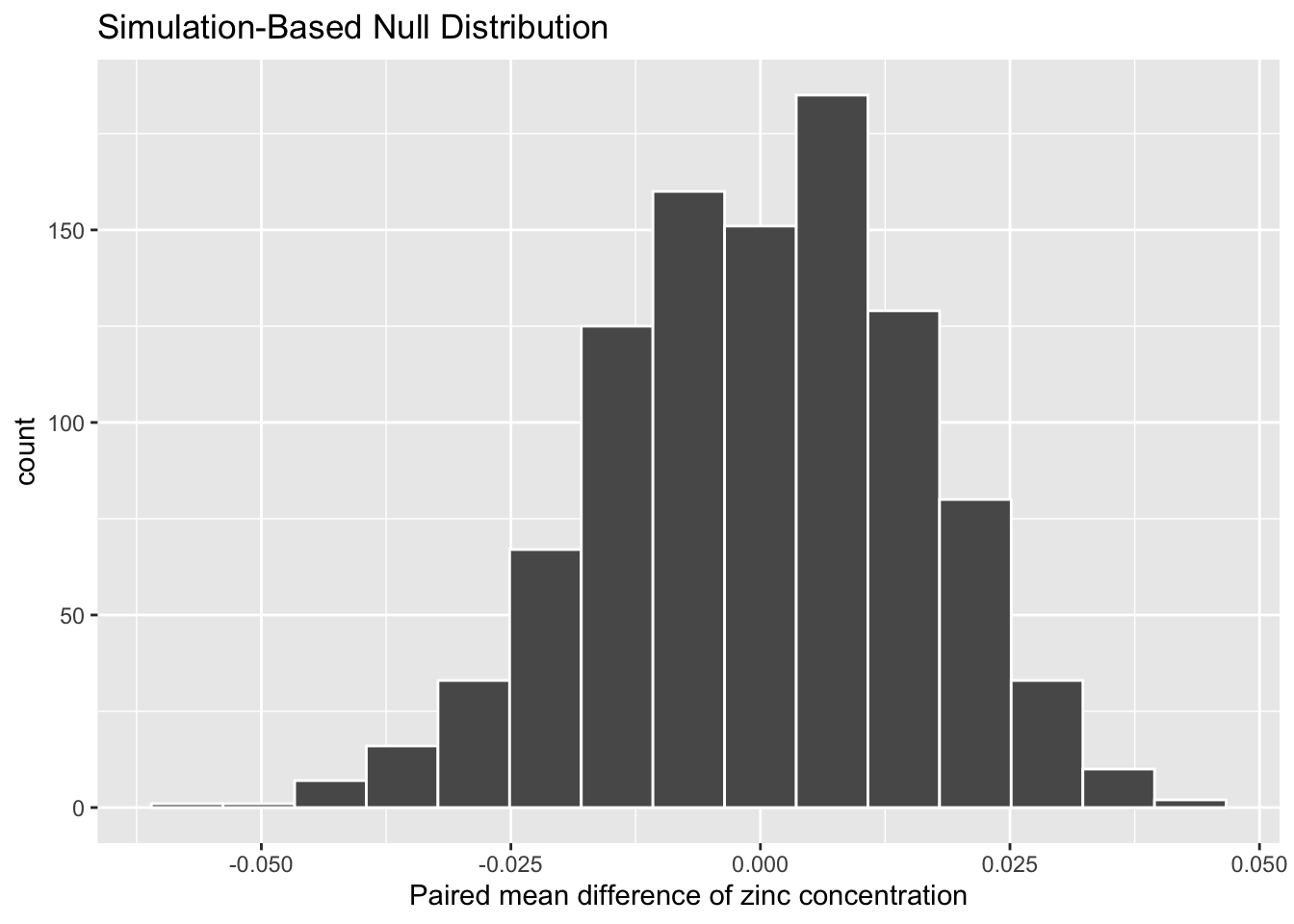
Figure B.7: Bootstrap distribution for zinc concentraion differences.
We can next use this distribution to observe our \(p\)-value. Recall this is a left-tailed test (\(H_A: \mu_{diff} < 0\)), so we will be looking for values that are less than or equal to -0.0804 for our \(p\)-value.
infer::visualize(null_distn_paired_means) +
  infer::shade_p_value(obs_stat = d_hat, direction = "less")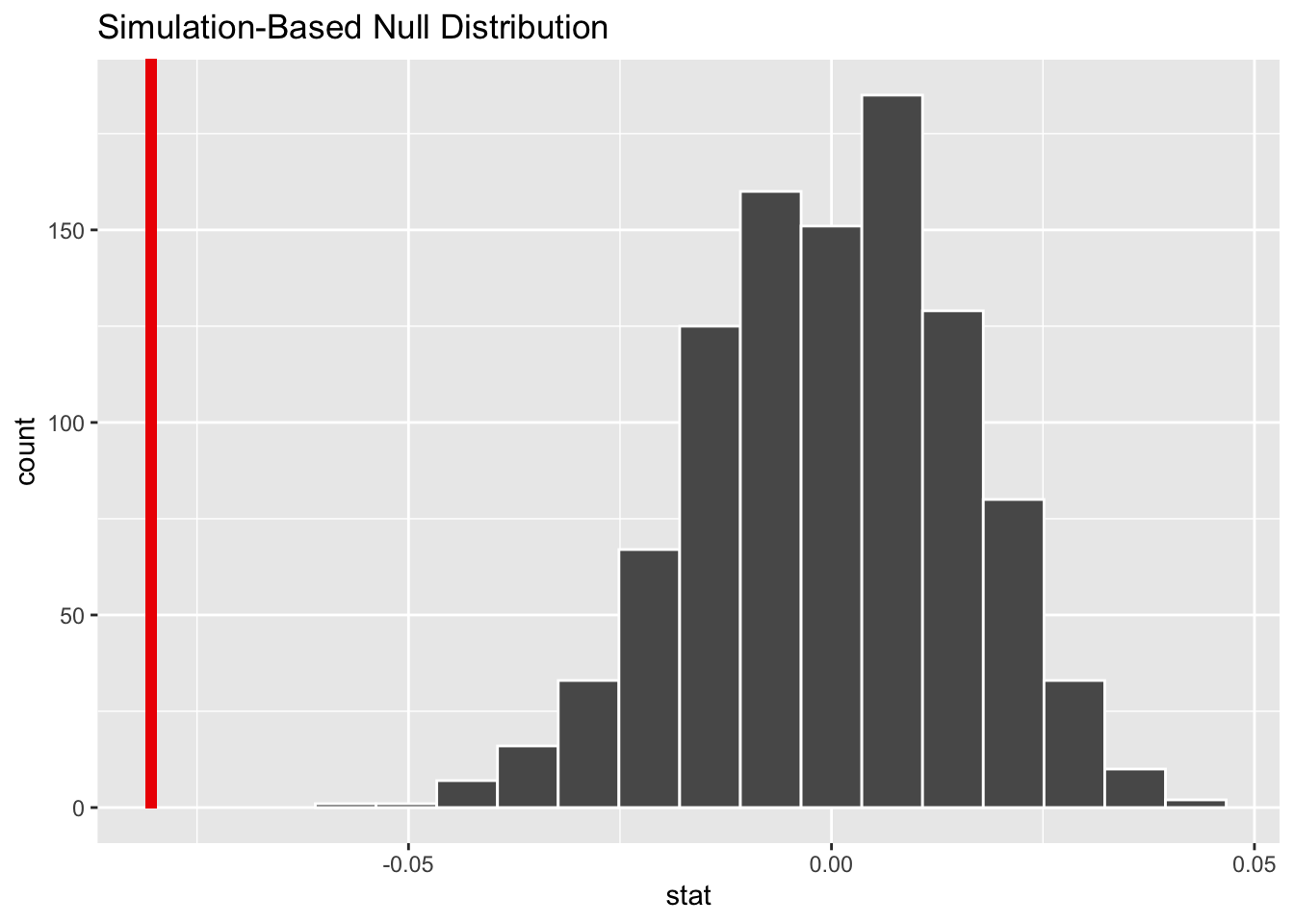
Figure B.8: Bootstrap distribution for zinc concentration differences; vertical red line = observed mean difference of 10 pairs of sample
Calculate \(p\)-value
pvalue <- null_distn_paired_means %>%
  infer::get_pvalue(obs_stat = d_hat, direction = "less")
pvalue
# A tibble: 1 x 1
p_value
<dbl>
1 0Similar to the previous example, you will have received a warning about \(p\)-value of 0. Instead of reporting that \(p\) is equal to zero, we can report \(p < 0.01\), and that we reject the null hypothesis at the 5% level. You can also see this from the histogram above that we are far into the left tail of the null distribution.
Bootstrapping for confidence interval
We can also create a confidence interval
for the unknown population parameter \(\mu_{diff}\)
using our sample data (the calculated differences) with bootstrapping.
This is similar to the bootstrapping done in a one sample mean case,
except now our data is differences instead of raw numerical data.
Note that this code is identical to the pipeline
shown in the hypothesis test above except the hypothesize() function is not called.
boot_distn_paired_means <- zinc_diff %>%
  infer::specify(response = pair_diff) %>%
  infer::generate(reps = 1000, type = "bootstrap") %>%
infer::calculate(stat = "mean")# A tibble: 1 x 2
lower_ci upper_ci
<dbl> <dbl>
1 -0.110 -0.0516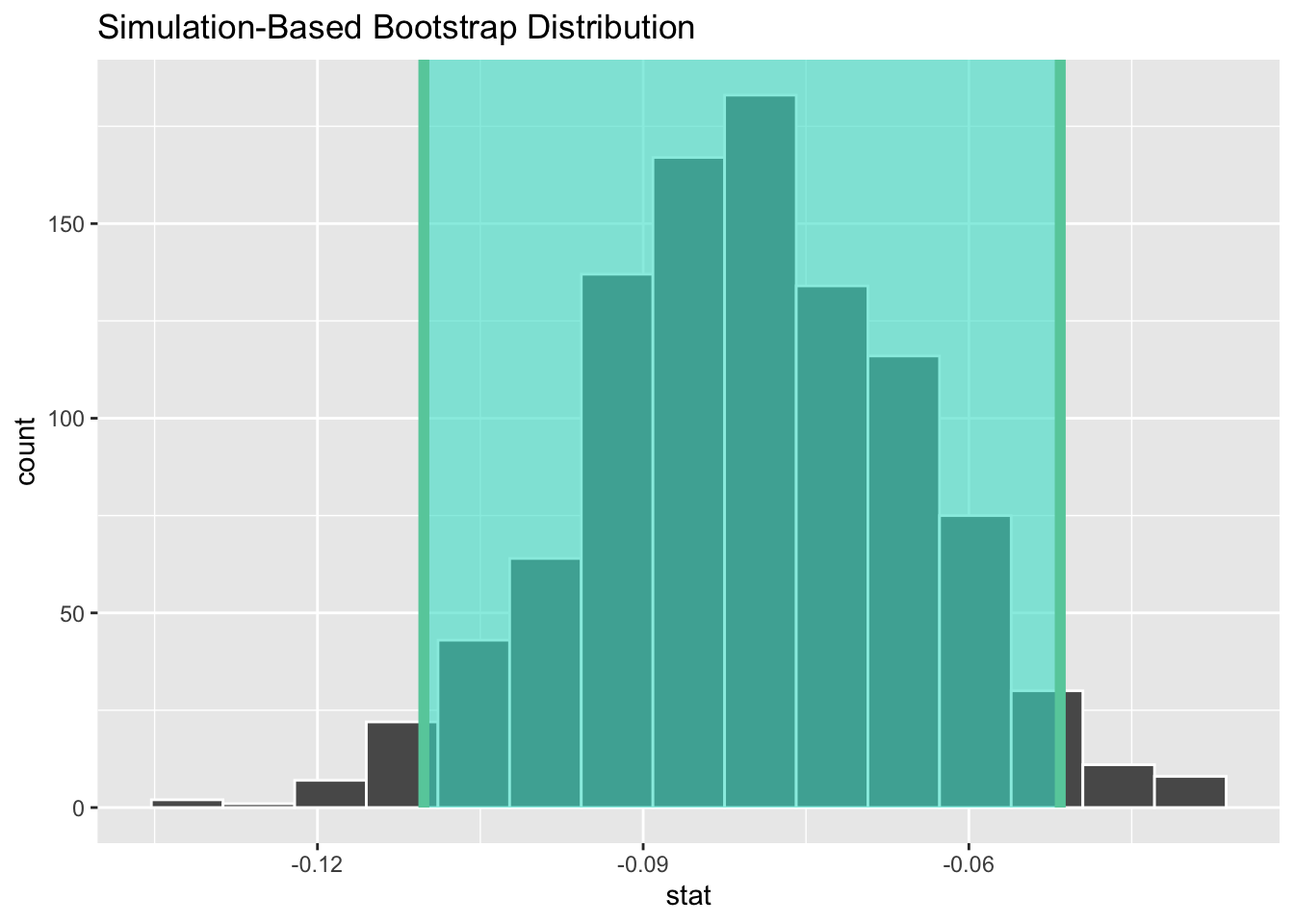
Figure B.9: A bootstrap 95% confidence interval for the zinc concentration difference between surface and bottom water.
We see that 0 is not contained in this confidence interval as a plausible value of \(\mu_{diff}\) (the unknown population parameter). This matches with our hypothesis test results of rejecting the null hypothesis. Given that zero is not a plausible value of the population parameter and that the entire confidence interval falls below zero, we have evidence that surface zinc concentration levels are lower, on average, than bottom level zinc concentrations.
Interpretation: We are 95% confident that the true mean zinc concentration on the surface is between 0.11 units to 0.05 units lower than on the bottom.
B.2.4 Theory-based methods
Check conditions
Remember that in order to use the shortcut (formula-based, theoretical) approach, we need to check that some conditions are met.
Independent observations: The observations among pairs are independent.
The locations are selected independently through random sampling so this condition is met.
Approximately normal: The distribution of population of differences is normal or the number of pairs is at least 30.
The histogram above does show some skew so we have reason to doubt the population being normal based on this sample. We also only have 10 pairs which is fewer than the 30 needed. A theory-based test may not be valid here.
Test statistic
As mentioned earlier, the data of interest consist of differences between pairs, and can be conceived as a single sample. The goal is to estimate the population mean difference \(\mu_{diff}\), so the test statistic is the sample mean, \(\bar{x}_{diff}\). We are testing how likely it is for us to have observed a sample mean of \(\bar{x}_{diff, obs} = 0.0804\) or larger assuming that the population mean difference is 0 (i.e., under the null hypothesis). If the conditions are met and assuming \(H_0\) is true, we can “standardize” this original test statistic of \(\bar{X}_{diff}\) into a \(t\)-statistic that follows a \(t\)-distribution with degrees of freedom equal to \(df = n - 1\), where \(n\) is the number of pairs:
\[ t =\dfrac{ \bar{x}_{diff} - 0}{ s_{diff} / \sqrt{n} } \sim t (df = n - 1) \]
where \(s\) represents the standard deviation of the sample differences and \(n\) is the number of pairs.
Observed test statistic
While one could compute this observed test statistic by “hand,”
the focus here is on the set-up of the problem
and in understanding which formula for the test statistic applies.
We can use the t_test function on the differences
to perform this analysis for us.
    One Sample t-test

data:  zinc_diff$pair_diff
t = -4.8638, df = 9, p-value = 0.0004456
alternative hypothesis: true mean is less than 0
95 percent confidence interval:
       -Inf -0.0500982
sample estimates:
mean of x
  -0.0804
We see here that the \(t_{obs}\) value is -4.86.
Compute \(p\)-value
The \(p\)-value—the probability of observing a \(t_{obs}\) value of -4.86 or less in our null distribution of a \(t\) with 9 degrees of freedom—is smaller than 0.01. This can also be calculated in R directly:
[1] 0.0004455656State conclusion
We, therefore, have sufficient evidence to reject the null hypothesis, \(t(9) = -4.86\), \(p < 0.001\). Our initial guess that our observed sample mean difference was not statistically less than the hypothesized mean of 0 has been invalidated here. Based on this sample, we have evidence that, on average, the mean concentration in the bottom water is greater than that of the surface water.
B.2.5 Comparing results
The results are similar for theory- and simulate-based methods in terms of the \(p\)-value and the confidence interval. The conditions for the theory-based method were not met because the number of pairs was smaller than 30, but the sample data were not highly skewed. Using either the theory-based or simulated-based method led to similar results here.
B.3 Two means (independent samples)
See Chapter 8
B.4 One proportion
B.4.1 Problem statement
The CEO of a large electric utility claims that 80 percent of his 1,000,000 customers are satisfied with the service they receive. To test this claim, the local newspaper surveyed 100 customers, using simple random sampling. 73 were satisfied and the remaining were unsatisfied. Based on these findings from the sample, can we reject the CEO’s hypothesis that 80% of the customers are satisfied? [Tweaked a bit from http://stattrek.com/hypothesis-test/proportion.aspx?Tutorial=AP]
B.4.2 Competing hypotheses
In words
Null hypothesis: The proportion of all customers of the large electric utility satisfied with service they receive is equal 0.80.
Alternative hypothesis: The proportion of all customers of the large electric utility satisfied with service they receive is different from 0.80.
In symbols (with annotations)
\(H_0: \pi = p_{0}\), where \(\pi\) represents the proportion of all customers of the large electric utility satisfied with service they receive and \(p_0\) is 0.8.
\(H_A: \pi \ne 0.8\)
Set \(\alpha\)
It’s important to set the significance level before starting the testing using the data. Let’s set the significance level at 5% here.
B.4.3 Exploring the sample data
# Let's create the data frame based on the problem statement
elec <- c(rep("satisfied", 73), rep("unsatisfied", 27)) %>%
  # use `tibble::enframe()` to convert vectors to data frames
  tibble::enframe() %>%
  dp$rename(satisfy = value)
The bar graph below also shows the distribution of satisfy.
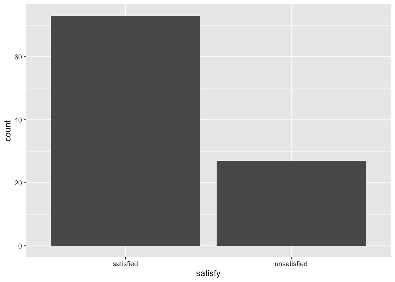
Figure B.10: Percentage of un/satisfied customers in a sample of 100.
The observed statistic is computed as
p_hat <- elec %>%
  infer::specify(response = satisfy, success = "satisfied") %>%
  infer::calculate(stat = "prop")
p_hat
# A tibble: 1 x 1
stat
<dbl>
1 0.73Guess about statistical significance
We are testing whether the sample proportion of 0.73 is statistically different from \(p_0 = 0.8\) based on this sample. They seem to be quite close, and our sample size is not huge here (\(n = 100\)). Let’s guess that we do not have evidence to reject the null hypothesis.
B.4.4 Simulation-based methods
Simulation for hypothesis test
To find out whether 0.73 is statistically different from 0.8, we need to account for the sample size. We also need to determine a process that replicates how the original sample of size 100 was selected. We can use the idea of an unfair coin to simulate this process. We will simulate flipping an unfair coin (with probability of success 0.8 matching the null hypothesis) 100 times. Then we will keep track of how many heads come up in those 100 flips. Our simulated statistic matches with how we calculated the original statistic \(\hat{p}\): the number of heads (satisfied) out of our total sample of 100. We then repeat this process many times (say 1,000) to create the null distribution looking at the simulated proportions of successes:
set.seed(2018)
null_distn_one_prop <- elec %>%
  infer::specify(response = satisfy, success = "satisfied") %>%
  infer::hypothesize(null = "point", p = 0.8) %>%
  infer::generate(reps = 1000) %>%
  infer::calculate(stat = "prop")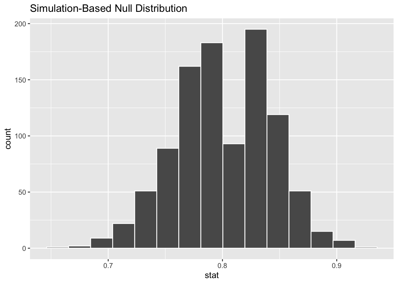
Figure B.11: Null distribution for percentage of satisfied customers.
We can next use this distribution to observe our \(p\)-value. Recall this is a two-tailed test so we will be looking for values that are 0.8 - 0.73 = 0.07 away from 0.8 in BOTH directions for our \(p\)-value:
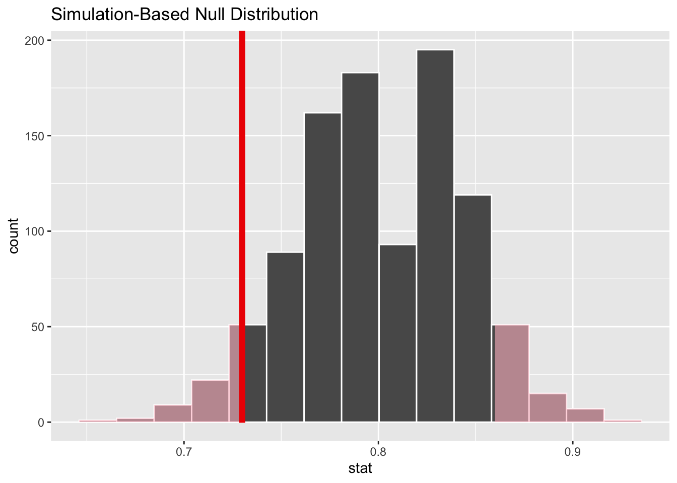
Figure B.12: Null distribution for percentage of satisfied customers; red vertical line = observed test statistic; two-tailed
Bootstrapping for confidence interval
We can also create a confidence interval for the unknown population parameter \(\pi\) using our sample data. To do so, we use bootstrapping, which involves
- sampling with replacement from our original sample of 100 survey respondents and repeating this process 1,000 times,
- calculating the proportion of successes for each of the 1,000 bootstrap samples created in Step 1.,
- combining all of these bootstrap statistics calculated in Step 2 into a
boot_distnobject, - identifying the 2.5th and 97.5th percentiles of this distribution (corresponding to the 5% significance level chosen) to find a 95% confidence interval for \(\pi\), and
- interpret this confidence interval in the context of the problem.
boot_distn_one_prop <- elec %>%
  infer::specify(response = satisfy, success = "satisfied") %>%
  infer::generate(reps = 1000) %>%
infer::calculate(stat = "prop")# A tibble: 1 x 2
lower_ci upper_ci
<dbl> <dbl>
1 0.63 0.82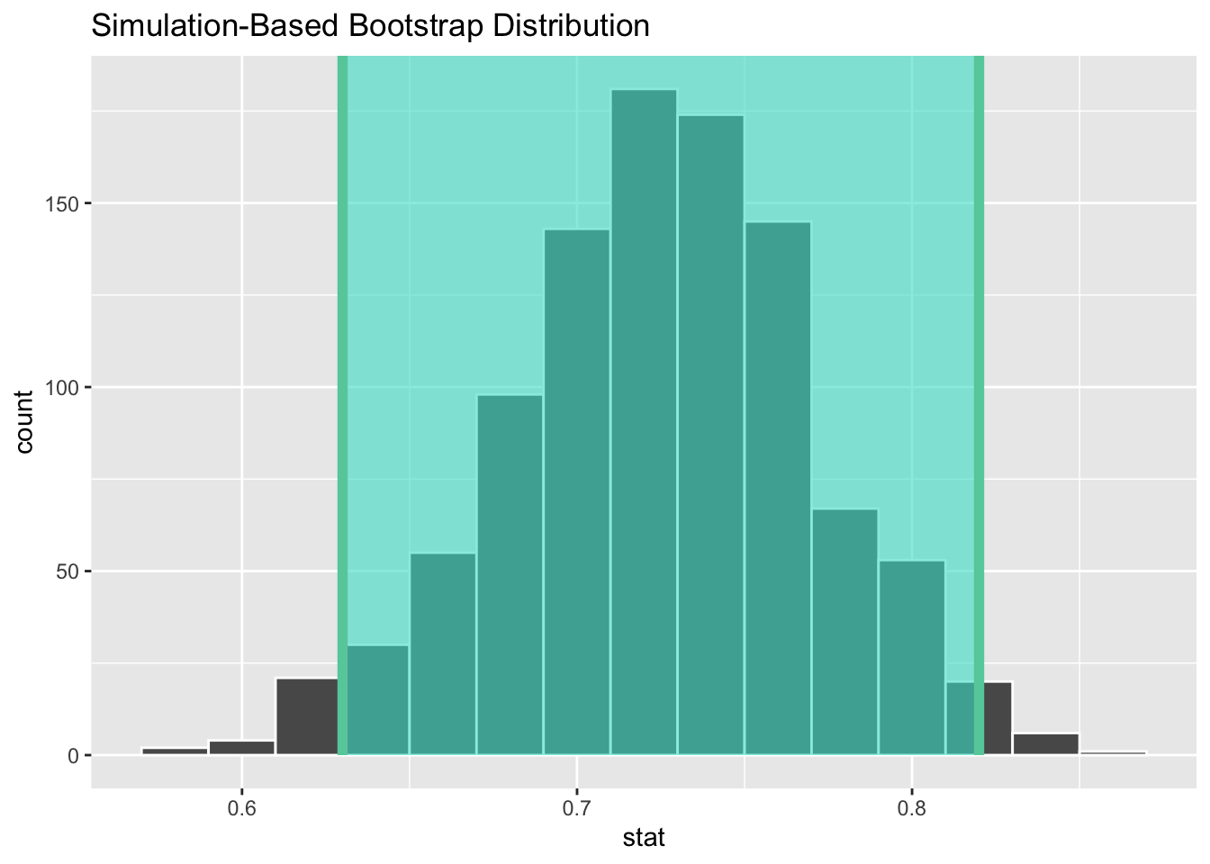
Figure B.13: A 95% confidence interval for percentage of satisfied customers.
We see that 0.80 is contained in this confidence interval as a plausible value of \(\pi\) (the unknown population proportion). This matches with our hypothesis test results of failing to reject the null hypothesis.
Interpretation: We are 95% confident that the true proportion of customers who are satisfied with the service they receive is between 0.63 and 0.82.
B.4.5 Theory-based methods
Check conditions
Remember that in order to use the shortcut (formula-based, theoretical) approach, we need to check that some conditions are met.
Independent observations: The observations are collected independently.
The cases are selected independently through random sampling so this condition is met.
Approximately normal: The number of expected successes and expected failures is at least 10.
This condition is met since 73 and 27 are both greater than 10.
Test statistic
Our goal is to test how likely it is for us to have observed a sample proportion of \(\hat{p}_{obs} = 0.73\) or larger assuming that the population proportion \(\pi\) is 0.80 (assuming the null hypothesis is true). If the conditions are met and assuming \(H_0\) is true, we can standardize this original test statistic of \(\hat{P}\) into a \(z\) statistic that follows a \(N(0, 1)\) distribution, i.e., a standard normal distribution with \(\mu = 0\) and \(\sigma = 1\).
\[ z =\dfrac{ \hat{p} - p_0}{\sqrt{\dfrac{p_0(1 - p_0)}{n} }} \sim N(0, 1) \]
Observed test statistic
While one could compute this observed test statistic by “hand” by plugging the observed values into the formula, the focus here is on the set-up of the problem and in understanding which formula for the test statistic applies. The calculation has been done in R below for completeness though:
[1] -1.75We see here that the \(z_{obs}\) value is around -1.75. Our observed sample proportion of 0.73 is 1.75 standard errors below the hypothesized parameter value of 0.8.
Visualize and compute \(p\)-value
null_distribution_satis <- elec %>%
  infer::specify(response = satisfy, success = "satisfied") %>%
  infer::hypothesize(null = "point", p = 0.8) %>%
  # For theory-based null distribution, stat is "z" instead of "prop"
  infer::calculate(stat = "z")
# visualize the theoretical null distribution
infer::visualize(null_distribution_satis, method = "theoretical") +
  infer::shade_p_value(obs_stat = z_obs, direction = "both")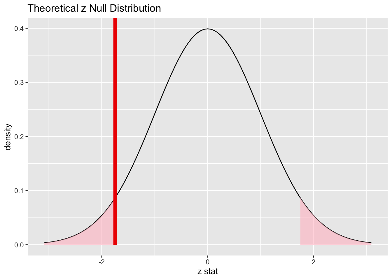
Figure B.14: Theory-based null distribution for percentage of satisfied customers.
[1] 0.08011831The \(p\)-value—the probability of observing an \(z_{obs}\) value of -1.75 or more extreme (in both directions) in our null distribution—is around 8%.
Note that we could also do this test directly using the prop.test function.
prop.test(
  x = table(elec$satisfy),
  n = length(elec$satisfy),
  alternative = "two.sided",
  p = 0.8,
  correct = FALSE
)
    1-sample proportions test without continuity correction

data:  table(elec$satisfy), null probability 0.8
X-squared = 3.0625, df = 1, p-value = 0.08012
alternative hypothesis: true p is not equal to 0.8
95 percent confidence interval:
 0.6356788 0.8073042
sample estimates:
   p
0.73
prop.test does a \(\chi^2\) test here but this matches up exactly
with what we would expect: \(\chi^2_{obs} = 3.06 = (-1.75)^2 = (z_{obs})^2\)
and the \(p\)-values are the same because we are focusing on a two-tailed test.
Note that the 95 percent confidence interval given above matches well with the one calculated using bootstrapping.
State conclusion
We, therefore, do not have sufficient evidence to reject the null hypothesis, \(\chi^2_{obs} = 3.06\), \(p = 0.08\). Based on this sample, we do not have evidence that the proportion of all customers of the large electric utility satisfied with service they receive is different from 0.80, at the \(\alpha = 0.05\) level.
B.5 Two proportions
See Chapter 7.