Chapter 9 Effect Size and Power
So far in this course, we have been focusing on what to do AFTER data have been collected: visualize, tidy, infer (generalize). In this chapter, let’s shift our focus and consider what to do BEFORE data are even collected. Although most introductory statistics books dedicate most of their space to what happens AFTER data collection, it does not mean that what happens before data collection is any less important. Quite the opposite. Data collected without careful planning could result in many undesirable consequences including:
- being forced to use suboptimal analytical tools,
- wasting time and resources,
- invalid conclusions,
- regret.
One of the reasons why textbooks do not open with how to plan data collection is because the planning phase requires one to consider, for example, effect size and power — concepts that build up on more basic ones such as standard error (Chapter 5) confidence intervals (Chapter 6), Type I and Type II errors (Chapter 7). Now that you have mastered those basic concepts, it is time to learn how to plan data collection; in particular, how many participants you would need to recruit.
Good to know
Planning a study
The proverb “failing to plan is planning to fail” certainly applies to research as well as everyday life. Planning a study typically starts with formulating a reseasrch question. The question might be inspired by studying a body of literature, conversing with a colleague, attending a seminar, … or a combination of any of them. Once a research question is born, in theory, it will dictate which analytical tool to use. In practice, however, we tend to pursue only questions that seem feasible given the tools we are already familiar with — yet another chicken and egg problem. Or as the famous saying goes,
If your only tool is a hammer then every problem looks like a nail.
The bottom line is, we should make a genuine effort to pose the most relevant question, rather than forcing the question to fit into the methodology framework we are comfortable with.
Once we have decided on the research question and what analytical tools to apply, the next step would be deciding how many participants to recruit given the anticipated findings. This is the focus of the current chapter.
Needed packages
Let’s get ready all the packages we will need for this chapter.
# Install xfun so that I can use xfun::pkg_load2
if (!requireNamespace('xfun')) install.packages('xfun')
xf <- loadNamespace('xfun')

cran_packages <- c(
                  "dplyr",
                  "esc", # a new package we will introduce in this chapter
                  "ggplot2",
                  "infer",
                  "skimr",
                  "tibble",
                  "tidyr"
)

if (length(cran_packages) != 0) xf$pkg_load2(cran_packages)

gg <- import::from(ggplot2, .all=TRUE, .into={new.env()})
dp <- import::from(dplyr, .all=TRUE, .into={new.env()})

import::from(magrittr, "%>%")
import::from(patchwork, .all=TRUE)
9.1 Pip and Max
Let’s revisit the second example you have seen in Chapter 8. Recall that a new graudate was deciding where to re-locate and was basing his decision on income prospects of the destinations. Let’s call this person Pip. Using US Census data, Pip compared the average income between Cleveland, Ohio, and Sacramento, California.
# retrieve the sample Pip drew
pip_cle_sac <- read.delim("https://moderndive.com/data/cleSac.txt") %>%
  dp$rename(
    income = Total_personal_income
  ) %>%
    dp$mutate(
    metro_area = as.factor(Metropolitan_area_Detailed)
        ) %>%
  dp$select(income, metro_area) %>%
  na.omit()
tibble::glimpse(pip_cle_sac)
Rows: 387
Columns: 2
$ income <int> 40240, 13600, 0, 49000, 38300, 14000, 9000, 40000, 18000, …
$ metro_area <fct> Sacramento_ CA, Sacramento_ CA, Sacramento_ CA, Sacramento…Let’s say that another person, Max, used the same strategy to help decide where to re-locate after graduation. It just so happens that Max is also choosing between Cleveland, Ohio, and Sacramento, California. Unlike Pip, however, Max obtained a larger sample from the same pool, the US Census data.
# retrieve the sample Max drew
max_cle_sac <- dget("https://raw.githubusercontent.com/chunyunma/baby-modern-dive/master/data/max_cle_sac.txt")
tibble::glimpse(max_cle_sac)
Rows: 1,935
Columns: 2
$ income <int> 16000, 44800, 13900, 60000, 13400, 62000, 160000, 0, 50000…
$ metro_area <fct> Sacramento_ CA, Sacramento_ CA, Sacramento_ CA, Cleveland_…9.1.1 Exploring both samples
In Chapter 8, we have already conducted exploratory analysis on Pip’s data. Nevertheless, let’s run summary statistics and boxplots on both Pip’s and Max’s data for comparison.
# Create a template function for descriptives
my_skim <- skimr::skim_with(base = skimr::sfl(n = length, missing = skimr::n_missing),
                     numeric = skimr::sfl(
                                          mean,
                                          sd,
                                          iqr = IQR,
                                          min,
                                          p25 = ~ quantile(., 1/4),
                                          median,
                                          p75 = ~ quantile(., 3/4),
                                          max
                                          ),
                            append = FALSE
) #sfl stands for "skimr function list"
# summary statistics for Pip's sample
pip_cle_sac %>%
dp$group_by(metro_area) %>%
my_skim(income) %>%
skimr::yank("numeric") %>%
knitr::kable(
caption = "Summary statistics for Pip's sample"
)| skim_variable | metro_area | n | missing | mean | sd | iqr | min | p25 | median | p75 | max |
|---|---|---|---|---|---|---|---|---|---|---|---|
| income | Cleveland_ OH | 212 | 0 | 27467.07 | 27680.68 | 26800 | 0 | 8475 | 21000 | 35275 | 152400 |
| income | Sacramento_ CA | 175 | 0 | 32427.54 | 35773.63 | 41300 | 0 | 8050 | 20000 | 49350 | 206900 |
# summary statistics for Max's sample
max_cle_sac %>%
  dp$group_by(metro_area) %>%
  my_skim(income) %>%
  skimr::yank("numeric") %>%
  knitr::kable(
               caption = "Summary statistics for Max's sample"
)| skim_variable | metro_area | n | missing | mean | sd | iqr | min | p25 | median | p75 | max |
|---|---|---|---|---|---|---|---|---|---|---|---|
| income | Cleveland_ OH | 1045 | 0 | 28327.56 | 27657.13 | 26000 | 0 | 9000 | 23200 | 35000 | 152400 |
| income | Sacramento_ CA | 890 | 0 | 32145.28 | 35327.89 | 37475 | 0 | 7325 | 22600 | 44800 | 206900 |
The boxplot below also shows the mean for each group highlighted by the red dots.
pip_boxplot_income <- pip_cle_sac %>% gg$ggplot(gg$aes(x = metro_area, y = income)) +
  gg$geom_boxplot() +
  gg$stat_summary(fun = "mean", geom = "point", color = "red") +
  gg$labs(subtitle = "Pip's sample; n = 387")

max_boxplot_income <- max_cle_sac %>% gg$ggplot(gg$aes(x = metro_area, y = income)) +
  gg$geom_boxplot() +
  gg$stat_summary(fun = "mean", geom = "point", color = "red") +
  gg$labs(subtitle = "Max's sample; n = 1935")

pip_boxplot_income + max_boxplot_income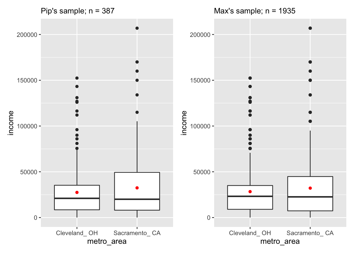
Figure 9.1: CAPTION
Except for the obvious sample size difference, both Pip’s and Max’s data exhibit similar pattern. The average income for both Cleveland and Sacramento are comparable cross Pip’s and Max’s sample; so are the ranges.
Guess about statistical significance
From Section 8.2, we already know that Pip’s data failed to reject the null hypothesis, that his data did not provide enough evidence to support the notion that the true mean income differed between Cleveland and Sacramento. Therefore, average income was not a useful criterion for Pip to choose between the two cities. Given the similar distributions of data in both Pip’s and Max’s sample, as shown in Figure 9.1, we have no reason to believe that Max’s data would lead to a different conclusion. In other words, we suspect that Max will also need to drop income as a criterion in his pro-and-con list.
Recall from Chapter 8 that both theory-based and simulated-based methods led to highly similar results for Pip’s data. For brevity, let’s apply theory-based methods, i.e., two sample \(t\)-tests to both Pip’s and Max’s data in this chapter.
9.1.2 Competing hypotheses
In words
Null hypothesis: The mean income is the same for both cities.
Alternative hypothesis: The mean income is different for the two cities.
In symbols (with annotations)
\(H_0: \mu_{sac} = \mu_{cle}\) or \(H_0: \mu_{sac} - \mu_{cle} = 0\), where \(\mu\) represents the average income.
\(H_A: \mu_{sac} - \mu_{cle} \ne 0\)
9.1.3 Check conditions
From Section 9.1.3, we have confirmed that Pip’s data met the conditions for theory-based methods. Let’s check Max’s data now.
Independent observations: The observations are independent in both groups.
This condition is met because the cases are randomly selected from each city.
Approximately normal: The distribution of the response for each group should be normal or the sample sizes should be at least 30.
gg$ggplot(max_cle_sac, gg$aes(x = income)) +
  gg$geom_histogram(color = "white", binwidth = 20000) +
  gg$facet_wrap(~metro_area)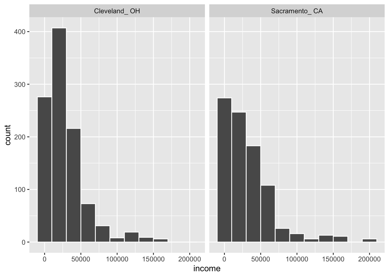
Figure 9.2: Distributions of income in two cities for Max’s sample.
We have some reason to doubt the normality assumption here because both histograms deviate from a standard normal curve. The sample sizes for each group are well over 100 though so the assumptions should still apply.
Independent samples: The samples should be collected without any natural pairing.
There is no mention of there being a relationship between those selected in Cleveland and in Sacramento.
9.1.4 Two-sample \(t\)-test
Test statistic
We have seen the theory-based test statistic for Pip’s data, which is a \(t\)-statistic by standardizing the difference in sample means (\(\bar{x}_{sac} - \bar{x}_{cle}\)):
\[ t = \frac{ (\bar{x}_{sac} - \bar{x}_{cle}) - (\mu_{sac} - \mu_{cle})}{ \text{SE}_{\bar{x}_{sac} - \bar{x}_{cle}} } = \dfrac{ (\bar{x}_{sac} - \bar{x}_{cle}) - 0}{ \sqrt{\dfrac{{s_{sac}}^2}{n_{sac}} + \dfrac{{s_{cle}}^2}{n_{cle}}} } \sim t (df = n_{sac} + n_{cle} - 2) \]
where \(n_{sac} = 175\) for Sacramento and \(n_{cle} = 212\) for Cleveland.
An almost identical test statistic applies to Max’s data:
\[ t = \frac{ (\bar{x}_{sac} - \bar{x}_{cle}) - (\mu_{sac} - \mu_{cle})}{ \text{SE}_{\bar{x}_{sac} - \bar{x}_{cle}} } = \dfrac{ (\bar{x}_{sac} - \bar{x}_{cle}) - 0}{ \sqrt{\dfrac{{s_{sac}}^2}{n_{sac}} + \dfrac{{s_{cle}}^2}{n_{cle}}} } \sim t (df = n_{sac} + n_{cle} - 2) \]
where \(n_{sac} = 890\) for Sacramento and \(n_{cle} = 1045\) for Cleveland.
Observed \(t\)-scores and \(p\)-values
# $t$-test for Pip's sample
pip_t_test <-
  t.test(income ~ metro_area, data = pip_cle_sac, alternative = "two.sided")
pip_t_test

# $t$-test for Max's sample
max_t_test <-
  t.test(income ~ metro_area, data = max_cle_sac, alternative = "two.sided")
max_t_test
    Welch Two Sample t-test

data:  income by metro_area
t = -1.5006, df = 323.36, p-value = 0.1344
alternative hypothesis: true difference in means is not equal to 0
95 percent confidence interval:
 -11463.712   1542.758
sample estimates:
 mean in group Cleveland_ OH mean in group Sacramento_ CA
                    27467.07                     32427.54


    Welch Two Sample t-test

data:  income by metro_area
t = -2.6132, df = 1671.5, p-value = 0.00905
alternative hypothesis: true difference in means is not equal to 0
95 percent confidence interval:
 -6683.1496  -952.2926
sample estimates:
 mean in group Cleveland_ OH mean in group Sacramento_ CA
28327.56 32145.28 | Sample | \(x_{sac} - x_{cle}\) | \(p\)-value | Conclusion |
|---|---|---|---|
| Pip’s | 4961 | 0.13 | Fail to reject \(H_0\) |
| Max’s | 3817 | 0.01 | Reject \(H_0\) |
Even though the absolute difference between the mean income of Cleveland and Sacramento in Pip’s sample (\(\bar{x}_{sac} - \bar{x}_{cle} = 4961\)) is similar to that in Max’s sample (\(\bar{x}_{sac} - \bar{x}_{cle} = 3817\)), the conclusion they would draw are drastically different. Based on Pip’s sample, we do not have sufficient evidence to reject the null hypothesis, \(t\)(385) = -1.5, \(p\) = 0.13. Pip would need to consider other criteria that can distinguish the two cities more unequivocally. In contrast, Max’s data would lead to rejection of the null hypothesis, \(t\)(1933) = -2.61, \(p\) = 0.01. For Max, Sacramento would seem a clearly favourable destination as far as income prospect is concerned.
How can we reconcile such drastic difference from two seemingly indistinguishable samples? If we call \(\bar{x}_{sac} - \bar{x}_{cle}\) a measure of the income difference’s magnitude, then what does \(p\) measure? A \(p\) value certainly does not measure the same construct as does \(\bar{x}_{sac} - \bar{x}_{cle}\). Otherwise, the slightly more pronounced income difference in Pip’s sample (\(\bar{x}_{sac} - \bar{x}_{cle} = 4961\), compared to \(\bar{x}_{sac} - \bar{x}_{cle} = 3817\) for Max’s sample) should have had a slightly higher chance of rejecting the null hypothesis, opposite to what happened in reality.
A \(p\) value measures the rarity of the observed statistic under the null hypothesis. Recall in Section 7.1.4, to test whether female candidates faced disadvantages due to gender discrimination, we used shuffling/permutation to simulate 1,000 samples under the null hypothesis. From these 1,000 simulated samples, we were able to construct a null distribution (Figure 7.5). Then comparing the observed statistic — 29.2% — to the null distribution, we asked ourselves: how likely it is to observe a promotion difference between male and female candidates as extreme as or more extreme than 29.2% under the null hypothesis? Of the 1,000 simulated samples, 6 of them returned a result as big as or larger than 29.2%. Six out of one-thousand, 6/1000, or less than 1%, is considerably smaller than our predefined threshold \(\alpha = 0.05\), which led us to reject the null hypothesis. We designate \(p\) the rarity, or the proportion of observing a test statistic just as extreme or more extreme than the observed test statistic under the null hypothesis.
Good to know
When people are presented with two different \(p\) values, they natually tend to compare the sizes of them, and claim “one result is more significant than the other.” Being significant is a binary status; a result is either significant or not. There is no such thing as “more significant or less significant”.
If you must compare the sizes of two \(p\) values — an understanble impulse but completely unnecessary, be prepared to embrace all the parenthetical remarks. For example,
The result observed by Max is more rare (sample size \(n = 1935\)) than that observed by Pip (sample size \(n = 387\)), given the null hypothesis that there is no income difference between Cleveland and Sacramento (\(\alpha = 0.05\)).
Once you have understood what a \(p\)-value can and cannot tell us — a \(p\)-value can tell us how rare an observed result is given the null hypothesis, but not the magnitude of the effect — it becomes obvious why Max’s and Pip’s samples led to different conclusions despite their similarity. Max has a much larger sample size (\(n = 1935\), five-times as many to be exact) than Pip (\(n = 387\)). Therefore, a difference of $3,817 from Max’s sample would be relatively more rare compared to the remaining \(1900+\) numbers under the null hypothesis, hence a smaller \(p\)-value, small enough to reject \(H_0\).
9.2 Effect size
Although \(\bar{x}_{sac} - \bar{x}_{cle}\) provides an intuitive measure of the income difference’s magnitude, it is hard to compare such measures across studies, especially when income is meausured in different units in each study: $ (US dollar), € (Euro), ¥ (Yen) … A standardized effect size provides a unit-free measurement of an effect’s magnitude which can be compared across studies. Effect is used here as the generic term for any quantity that is the target of an analysis: a mean, a difference between means, a correlation coefficient, a regression coefficient, etc. There are as many as 50 to 100 types of standardized effect size. We will introduce a few of them in this course, one at a time.
A commonly used effect size for two-sample \(t\)-tests is Cohen’s \(d\) (Cohen 1988). To understand how effet sizes work, let’s take a look at its formula. Applying Cohen’s \(d\) to the current example, we have
\[ \text{estimated Cohen's } d = \dfrac{\bar{x}_{sac} - \bar{x}_{cle}}{s_{pooled}} \tag{9.1} \]
where
\[ s_{pooled} = \sqrt{\dfrac{(n_{sac} - 1)s_{sac}^2 + (n_{cle} - 1)s_{cle}^2}{n_{sac} + n_{cle} - 2}} \]
Let’s zoom in on Equation (9.1). In the numerator, we have the absolute magnitude of income difference. \(s_{pooled}\) in the denominator is called the pooled standard deviation, which can be conceived as the common variation by pooling information from Sacramento’s income sample and Cleveland’s income sample. You can think of of the denominator as a scaler for the numerator, so as to make it comparable across studies, irrespective of the unit used in a specific study.
Cohen suggested some rule of thumb for evaluating the size of \(d\) (Cohen 1988):
\(d\) = 0.2, small
\(d\) = 0.5, medium
\(d\) = 0.8, large
This rule of thumb has been amended by other researchers to include the following (Sawilowsky 2009):
\(d\) = 1.2, very large
\(d\) = 2.0, huge
9.2.1 Caculate effect size using esc package
Let’s calculate the effect size for both Pip’s and Max’s sample.
Instead of doing it manually,
we can use function esc_t() from the esc package.
Most parameters in the est_c() function are fairly self-explanatory,
except the es.type = "g" on line 8.
Setting es.type to "g" means that we get Hedges’ \(g\) instead of Cohen’s \(d\).
Both Hedges’ \(g\) and Cohen’s \(d\) are standardized effect sizes
appropriate for two-sample \(t\)-test.
The only difference is that Hedges’ \(g\) is slightly less biased,
and thus preferable,
when the two said samples have different sample sizes.
Both Pip’s sample and Max’s sample have uneven number of observations
in two cities.
For example, in Pip’s sample, \(n_{cle} = 212\),
\(n_{sac} = 175\).
Therefore, we opted for Hedges’ \(g\) by setting es.type to "g", instead of
"d".
Note that the rule of thumb we introduced earlier based on Cohen’s \(d\)
still applies to Hedges’ \(g\).
To calculate Hedges’ \(g\) for Pip’s sample:
pip_cleveland <- pip_cle_sac %>% dp$filter(metro_area = "Cleveland_ OH")
pip_sacramento <- pip_cle_sac %>% dp$filter(metro_area = "Sacrament_ CA")

esc::esc_t(t = pip_t_test$statistic,
                         totaln = nrow(pip_cle_sac),
                         grp1n = nrow(pip_cleveland),
                         grp2n = nrow(pip_sacramento),
                         es.type = "g")$es %>%
  round(3) %>%
  abs()
t
0.152 Hedges’ \(g\) for Max’s sample:
max_cleveland <- max_cle_sac %>% dp$filter(metro_area = "Cleveland_ OH")
max_sacramento <- max_cle_sac %>% dp$filter(metro_area = "Sacrament_ CA")

esc::esc_t(t = max_t_test$statistic,
                         totaln = nrow(max_cle_sac),
                         grp1n = nrow(max_cleveland),
                         grp2n = nrow(max_sacramento),
                         es.type = "g")$es %>%
  round(3) %>%
  abs()
t
0.119 | Sample | \(x_{sac} - x_{cle}\) | Hedges g | \(p\)-value | Conclusion |
|---|---|---|---|---|
| Pip’s | 4961 | 0.152 | 0.13 | Fail to reject \(H_0\) |
| Max’s | 3817 | 0.119 | 0.01 | Reject \(H_0\) |
Contrary to the drastically different \(p\)-values in two samples,
the effect sizes in two sample are quite comparable
(0.152 and 0.119).
Despite the tiny \(p\) value in Max’s sample
(\(p\) = 0.009 is very significant,
as one may be tempted to conclude but should not),
the effect size remains unchaged and, using Cohen’s rule of thumb,
is considered to be small.
This result demonstrates the importance of reporting
both statistical significance and effect size,
as they complement each other.
9.3 Planning a study
Now that we have compared Pip’s and Max’s sample through the lens of effect size, let’s look at an important application of effect size: helping researchers plan the sample size of a study.
To find out how large a study’s sample should be, the researcher must have the following four ingredients ready (Huck 2016):
The type of statistical test the researcher plans to use to analyze the to-be-collected data, including the decision of one-tailed vs. two-tailed if applicable
The significance level (\(\alpha\) value)
The desired level of statistical power (\(1 - \beta\))
The a priori effect size
Type of statistical test. The required sample size is tied to the type of statistical test you plan to use. There is not a universal magic number that you can use as the sample size. As a general rule of thumb, a repeated measure design requires fewer participants than a between-subject design. Each test has its pros and cons. You should let the research question drive which test to use.
Significance level, a.k.a, \(\alpha\) level. Recall from Section 7.5.3, we mentioned that \(\alpha\) represents the probability of falsely rejecting a null hypothesis when it is in fact true (Type I error). To minimize the probability of making such an error, we often set \(\alpha\) to a very small value such as 0.05 or 0.01. For most social science, researchers follow domain-specific conventions in setting this parameter. For example, within psychology, 0.05 is the most common choice. However, being common is not equal to being true. As a general rule of thumb, if a study is exploratory and has a relatively small sample size, it is not unheard of to use a more liberal \(\alpha\) level such as 0.1. Alternatively, if a study has an impressive sample size and involve more than a handful of statistical tests, then every additional test contributes to an increasing chance of Type I error. As a remedy, reseachers use a more stringent \(\alpha\) level, say 0.01, for each individual test.
Statistical power. Recall from Section 7.5.3, we described statistical power as the probability of correctly rejecting a null hypothesis, represented by \(1 - \beta\), where \(\beta\) is the probability of making an error opposite to \(\alpha\) (Type II error). In most behavioural research, \(\beta\) is often set to 0.10 - 0.20, which results in a power between 0.8 and 0.9 (Cohen 1988, 56).
\[ \text{Power} = P(\text{Rejct} H_0 \mid H_0 \text{False}) \]
Effect Size. Selecting an appropriate a priori effect size is the most difficult aspect of sample size planning. A good rule of thumb: use a minimally meaningful effect size or the smallest effect size of interest, an effect size that you would hate to miss. It is okay if the observed effect size ends up being larger in the actual study. Using such theoretically driven effect sizes, one can calculate an upper bound of sample size needed, given the desirable power (\(1 - \beta\)) and significance (\(\alpha\)) levle.
Good to know
How to choose an appropriate a priori effect size?
A common practice among social science researchers is to conduct a pilot study before the main one. These pilot studies often use a small sample size. Like a dress rehearsal, a pilot study can be very useful for catching any kinks that may exist in the study plan. By definition, a pilot study is often highly similar to the main one. Therefore, researchers sometimes rely on results from a pilot study to estimate the effect size, which then becomes the input in calculating the sample size for the main study.
Albers and Lakens (2018) recommended against this practice. According to the authors’ simulation study, an effect size estimated from a pilot study is often biased due to its small sample size. The biased effect size will in turn lead to an under-estimated sample size, hence an underpowered main study. Instead, Albers and Lakens (2018) recommended that we use a minimally meaningful effect size, a.k.a. the smallest effect size of interest. Using this theoretically driven effect size, one can calculate an upper bound of sample size needed, given the desirable power (\(1 - \beta\)) and \(\alpha\) level. Optionally, one can use sequential analysis, wherein a few analyses can be planned in advance during data collection. For example, if a conservative estimate of the sample size is 400, then the researcher could decide, in advance, to analyze the data when n has reached 100, 200, 300, and 400. At any point, if the intended results have been achieved, data collection could terminate.
This post drew a similar conclusion, with a more nuanced discussion.
In the context of the income difference between Sacarmento and Cleveland, how much difference would you consider meaningful for income prospect to be a criterion in choosing between jobs? Although it is relatively easy to settle on a figure in the unit of $, say, five grand or ten grand, keep in mind that it is the standardized effect size that we need in order to find out the required sample size. We could either convert the dollar value to a standardized effect size using Equation (9.1), or choose a minimally meaningful effect size directly, say \(d = 0.3\).
Let’s say a difference of ten-thousand dollars is the miminal difference you would consider for choosing one city over the other. To standardize $10,000 using Equation (9.1), we also need to have access to \(s_{pooled}\), the pooled standard deviation. However, the current premise is that we are still in the planning phase and have not collected any data yet. Without a sample, we would not be able to estimate \(s_{pooled}\). Without \(s_{pooled}\), we are back to square one with choosing a minimally meaningful effect size.
This is a common predicament many researchers face when planning their study. And that’s why a theoretically-driven effect size is preferable. Let’s assume that, as a new graduate, we are sensitive to even a small-ish difference in income prospect, and choose \(d = 0.3\).
Table 9.5 lists all four ingredients of sample size planning for the current example:
| Ingredients | Values | Comments |
|---|---|---|
| Type of statistical test | Two-sample \(t\)-test, two-sided | |
| Significance level | \(\alpha = 0.05\) | Following convention |
| Power | \(1 - \beta = 0.8\) | Following convention |
| Effect size | \(d = 0.3\) | See rationale in the text above |
Next, we can use function power.t.test(), a base R function,
to find out the minimal sample size required
to achieve the said power and effect size specificed
in Table 9.5.
power.t.test(n = NULL, d = 0.3, sig.level = 0.05, power = 0.8,
             type = "two.sample", alternative = "two.sided")
     Two-sample t test power calculation

              n = 175.3851
          delta = 0.3
             sd = 1
      sig.level = 0.05
          power = 0.8
    alternative = two.sided

NOTE: n is number in *each* group
To reach a power of 80%, we would need around 175 observations from each city to detect a small effect size of 0.3.
Note that Pip’s sample has already met the threshold of sample size: (\(n_{sac} = 175\), \(n_{cle} = 212\)). If the income difference between Sacramento and Cleveland, once standardized and stripped off its unit, were truly more prominent than \(d = 0.3\) in the population, the \(t\)-test would have detected it. The fact that Pip’s sample failed to reject the null hypothesis (\(p\) = 0.13) suggests that the income levels in two cities were less distinguishable than what we would deem meaningfully different.
What about Max’s sample? Had he conducted a similar analysis before collecting data, he would have used a more appropriate sample size and reached the same conclusion as Pip did.
9.4 Conclusion
In this chapter, we introduced a family of standardized effect sizes including Cohen’s \(d\) and Hedges’ \(g\). We demonstrated its usefulness in complementing \(p\) values and informing readers about an effect’s magnitude. In addition, we have also shown you how to plan the sample size of a study by setting the a priori effect size.
In the subsequent chapters, we will introduce a couple additional type of effect sizes, each one appropriate for a specific research design.
9.4.1 Additional resources
This visualization may help you better understand the relationship among \(\alpha\), power, effect size, and sample size.