Chapter 10 Analysis of Variance
ANalysis Of VAriance, or ANOVA, arguably the most ubiqutous method within behavioural research, is a family of statistical tests to examine the differences among means. In Chapter 8, we have already learned how to test the difference between two means, i.e., the average income difference between Cleveland, OH, and Sacramento, CA, using a two-sample \(t\)-test. In this chapter, we will introduce the simplest form of ANOVA, which would allow us to compare three sample means simultaneously, and thereby testing whether or not the corresponding population means are equal.
So far in the second part of this book on statistical inferences, we have been consistently introducing both simulation- and theory-based methods for constructing confidence intervals, and for hypothesis testing, prioritizing simulation- over theory-based methods whenever possible. In this chapter, we will shift the priority and emphasize on theory-based methods for ANOVA. There are two main reasons for this arrangement. First, although simulation-based methods are especially useful for complex ANOVA designs (e.g., multivariate analysis), it does not offer a huge advantage over theory-based methods for the simple ANOVA design, which is the topic of the current chapter. Second, ANOVA is such an ubiqutous method across fields within psychology and currently the majority of researchers still use theory-based methods when they apply ANOVA on their data. It is paramount that you learn the lingos your peers and supervisors speak — in this case, terminologies underlying the theory-based ANOVA framework. On balance, I decided to lead with a full example on ANOVA using theory-based methods. For completeness, I will still walk you through an example at the end of this chapter (Section 10.3.1) on how to conduct a simple ANOVA using simulation-based methods.
To begin, we will introduce the logic of ANOVA through a toy example. Understanding this logic is key to applying ANOVA using both simulation-based and theory-based methods.
Needed packages
Let’s get ready all the packages we will need for this chapter.
# Install xfun so that I can use xfun::pkg_load2
if (!requireNamespace('xfun')) install.packages('xfun')
xf <- loadNamespace('xfun')

cran_packages <- c(
                  "dplyr",
                  "effectsize", # a new package we will introduce in this chapter
                  "infer",
                  "plotrix", # a new package we will introduce in this chapter
                  "rstatix", # a new package we will introduce in this chapter
                  "skimr"
)

if (length(cran_packages) != 0) xf$pkg_load2(cran_packages)

gg <- import::from(ggplot2, .all=TRUE, .into={new.env()})
dp <- import::from(dplyr, .all=TRUE, .into={new.env()})

import::from(magrittr, "%>%")
import::from(patchwork, .all=TRUE)
10.1 A toy example
Suppose that a researcher is interested in cellphone and distracted driving. They examined driving performance under three different treatment conditions: no cellphone, a hands-free cellphone, and a hand-held cellphone. Three samples of participants are selected, five participants for each treatment condition, fifteen participants in total. The purpose of the study is to determine whether or not using a cellphone would affect driving performance adversely (adapted from Gravetter and Wallnau (2011a)).
The study generated the following data (Table 10.1). Each of the fifteen participants contributed one data point: an integer corresponding to one’s driving performance measured in a driving simulator. The bigger the number, the better the driving performance.
| No phone | Hand-held | Hands-free |
|---|---|---|
| 3 | 0 | 3 |
| 5 | 1 | 2 |
| 7 | 3 | 2 |
| 4 | 1 | 5 |
| 6 | 0 | 3 |
At a glance, the five participants in the no-phone condition seemed to drive better compared to participants either in the hand-held or in the hands-free condition. To validate our hunch based on visual inspection, let’s calculate the average driving performance score across five participants in each condition. They have been listed in Table 10.2.
distracted_driving <- tibble::tibble(
                        driving_score = c(
                                          3, 5, 7, 4, 6,
                                          0, 1, 3, 1, 0,
                                          3, 2, 2, 5, 3
                                          ),
                        condition = c(rep("no-phone", 5),
                                          rep("hand-held", 5),
                                          rep("hands-free", 5)
                                          )
                        )

distracted_driving %>%
  dp$group_by(condition) %>%
dp$summarize(mean_score = mean(driving_score))| No phone | Hand-held | Hands-free |
|---|---|---|
| 3 | 0 | 3 |
| 5 | 1 | 2 |
| 7 | 3 | 2 |
| 4 | 1 | 5 |
| 6 | 0 | 3 |
| \(\bar{X}_1 = 5\) | \(\bar{X}_2 = 1\) | \(\bar{X}_3 = 3\) |
The sample means seem to agree with our intuition. On average, participants in the no-phone condition scored the highest on their driving performance. Extending the competing hypotheses we have seen from previous chapters, we can also formulate the null and alternative hypothesis for the current study as the following:
In words
Null hypothesis: The population mean driving performance score is the same for all three conditions.
Alternative hypothesis: The population mean driving performance scores in three conditions are not all the same; at least one of the population mean driving performance score is different from the rest.
In symbols
\(H_0\): \(\mu_{no} = \mu_{hand-held} = \mu_{hands-free}\), where \(\mu\) represents the population mean driving performance score.
\(H_A\): Not all \(\mu\) are equal.
Based on the last row in Table 10.2, participants under the no-phone condition on average scored higher on their driving performance (\(\bar{X} = 5\)) compared to participants in both the hand-held condition (\(\bar{X} = 1\)) and the hands-free condition (\(\bar{X} = 3\)).
However, let’s not forget that none of the three conditions had five identical scores. The five individuals within any condition did not receive the same score, despite the fact that these five individuals received exactly the same treatment. For example, within the no-phone condition, one participant scored as high as a 7, whereas another participant only received a mediocre 3. If we want to attribute the 4 point variation between \(\bar{X} = 5\) and \(\bar{X} = 1\) to the difference between conditions: a hand-held phone, then how do we explain away the same amount of variation — 4 point — that exists between two participants in the same condition?
In the ANOVA’s lingo, the first type of variation — differences that COULD be attributed to different conditions — is termed between-treatment variance, and the second type of variation — differences that occure among participants from the same condition — is termed within-treatment variance. In general, the within-treatment variance is assumed to be random and unsystematic, i.e., due to sampling error.
Recall the null hypothesis states that the population mean driving performance scores for the three conditions are all the same. Under this hypothesis, the between-treatment variance that we observed in the data — \(\bar{X}_1 = 5\) vs. \(\bar{X}_2 = 1\) vs. \(\bar{X}_3 = 3\) — are simply due to naturally occurring differences existing between one sample and another, i.e., sampling error.
In an ANOVA test, between-treatment variance is pitted against within-treatment variance. The ratio between the two, also known as the \(F\)-ratio, forms the test statistic of an ANOVA test:
\[ F = \frac{\text{between-treatment variance}}{\text{within-treatment variance}} \]
Under the null hypothesis, the value of the \(F\)-ratio is expected to be nearly equal to 1.00, because both between-treatment variance and within-treatment variance are attributed to sampling error under the null hypothesis, and hence of similar size. However, if the between-treatment variance is substantially larger than the within-treatment variance, or \(F\)-ratio much larger than 1.00, we have evidence to reject the null hypothesis.
Good to know
Sources of within-treatment variance
Whenever a study employs ANOVA for data analysis, there is a good chance that participants in the study were exposed to various conditions, i.e., levels of a variable, and some observations were made about those participants under each condition. For example, in the present example on cellphone and distracted driving, fifteen participants were exposed to three different levels of distraction — minimal distraction (no phone), medium amount of distraction (hands-free phone), and maximum distraction (hand-held phone) — five in each level. Observations were made for each participant on their driving performance under their respective condition. By comparing those observations, researchers expect to find differences among them and attribute such differences to the manipulated variable — amount of distraction, thereby concluding along the line of “manipulating variable x had an effect on participants’ performance.” Within-treatment variance refers to any variation among data points that cannot be accounted for by the varying conditions in a study. This is why within-treatment variance is also referred to as the error term, or simply error. They are considered nuisance, random noise that happens naturally and needs to be filtered out. Two primary sources of within-treatment variance are individual differences and measurement errors.
Individual differences. Five participants received the same amount of distraction, say, in the no-phone condition. And yet their driving performance scores were not all the same. It is entirely possible that these five individuals had different driving experience / skills to begin with. Or some are more accustomed to a driving simulator than others. There are almost infinite number of possibilities as to why individuals, when exposed to the same condition, exhibit different behaviour. Within-treatment variance due to individual differences can be reduced in a laboratory environment, but can never be made to disappear.
Measurement errors. Even if individuals could respond in exactly the same way when exposed to the same condition, the measurement of their response may still not be perfectly consistent, which would result in within-treatment variance. For example, if the researcher who rates participants’ driving performance secretely believe that male drivers tend to be more skilled than female drivers, then the researcher will more likely rate male participants favourably, thereby introducing variance to the data beyond what varying conditions could account for. Carefully designed experiment protocols can keep obvious measurement errors at bay, but as long as human beings are involved in the measurement — e.g., designing or executing the measurement, measurement errors are unavoidable in reality.
10.1.1 \(F\)-statistic
In practice, between-treatment variance is calculated using Equation (10.1), and within-treatment variance using Equation (10.2).
\[ \begin{aligned} \text{between-treatment variance} &= \frac{SS_{between}}{df_{between}} = MS_{between} \\ &= \frac{\sum_{j = 1}^k n_j (\bar{X}_j - \bar{X})^2}{k - 1} \end{aligned} \tag{10.1} \]
where \(SS\) stands for sum of squares, \(df\) stands for degrees of freedom, \(MS\) stands for mean sum of squares, \(k\) is the number of conditions, \(\bar{X}_j\) is the mean for each group \(j\), and \(\bar{X}\) is the overall mean. For example, \(k = 3\) in the current toy example, because there are three distraction levels. \(\bar{X}_1 = 5\) and \(\bar{X} = \frac{(\bar{X}_1 + \bar{X}_2 + \bar{X}_3)}{3} = \frac{5 + 1 + 3}{3} = 3\).
\[ \begin{aligned} \text{within-treatment variance} &= \frac{SS_{within}}{df_{within}} = MS_{within} \\ &= \frac{\sum_{i, j} (X_{ij} - \bar{X}_j)^2}{N - k} \end{aligned} \tag{10.2} \]
where \(N = n_1 + n_2 + \cdots + n_k\) with \(n_j\) being the sample size of group \(j\), and \(X_{ij}\) is the \(i^{th}\) observation in group \(j\). For example, \(n_1 = n_2 = n_3 = 5\), and \(N = 5 + 5 + 5 = 15\), \(X_{12}\) is the \(1^{st}\) observation in the hand-held (\(2^{nd}\)) condition, and \(X_{12} = 0\).
Finally, \(F\)-ratio can be expressed as
\[ F = \frac{MS_{between}}{MS_{within}} \tag{10.3} \]
All of the information can be summarized in a table such as the following:
| Source | Sum of Squares | Degrees of Freedom | Mean Sum of Squares | \(F\) |
|---|---|---|---|---|
| Between | \(SS_B\) | \(df_B = k - 1\) | \(MS_B = SS_B \mathbin{/} df_B\) | \(MS_B \mathbin{/} MS_W\) |
| Within | \(SS_W\) | \(df_W = N - k\) | \(MS_W = SS_W \mathbin{/} df_W\) | |
| Total | \(SS_T\) | \(N - 1\) |
A sum of squares devided by its corresponding degrees of freedom returns the mean sum of squares. A rule of thumb for deciding the degrees of freedom is as follows: Total sum of squares always has \(N - 1\) degrees of freedome, because we have \(N\) observations that fluctuate around the global mean. There are \(k -1\) degrees of freedome for the treatment effect because there are \(k\) groups minus one side-constraint (\(\sum_{j = 1}^k (\bar{X}_j - \bar{X}) = 0\)).6 The remaining part, i.e., within-treatment variance, has \(N - 1 - (k - 1) = N - k\) degrees of freedom.
It can be mathematically proven that under the null hypothesis \(H_0\):
\[ F = \frac{MS_{between}}{MS_{within}} \sim F_{k-1, N-k} \]
where we denote by \(F_{n,m}\) the so-called \(F\)-distribution with \(n\) and \(m\) as its two degrees of freedom parameters, one for \(\text{between-treatment variance}\) on the numerator — \(k - 1\) where \(k\) is the number of conditions, and one for \(\text{within-treatment variance}\) on the denominator — \(N - k\) where \(N\) is the total number of observations.
Figure 10.1 shows three \(F\)-distributions with different degrees of freedom parameters. The exact shape of the \(F\)-distribution depends on the two degrees of freedom parameters. For any \(F\)-distribution with degrees of freedom on the numerator equal or larger than 3, it piles up around 1.00, and then tapers off to the right. Notice that \(F\) values are always non-negative numbers. This is expected, because \(F\) values are ratios of two variances, and a variance by definition is never negative.
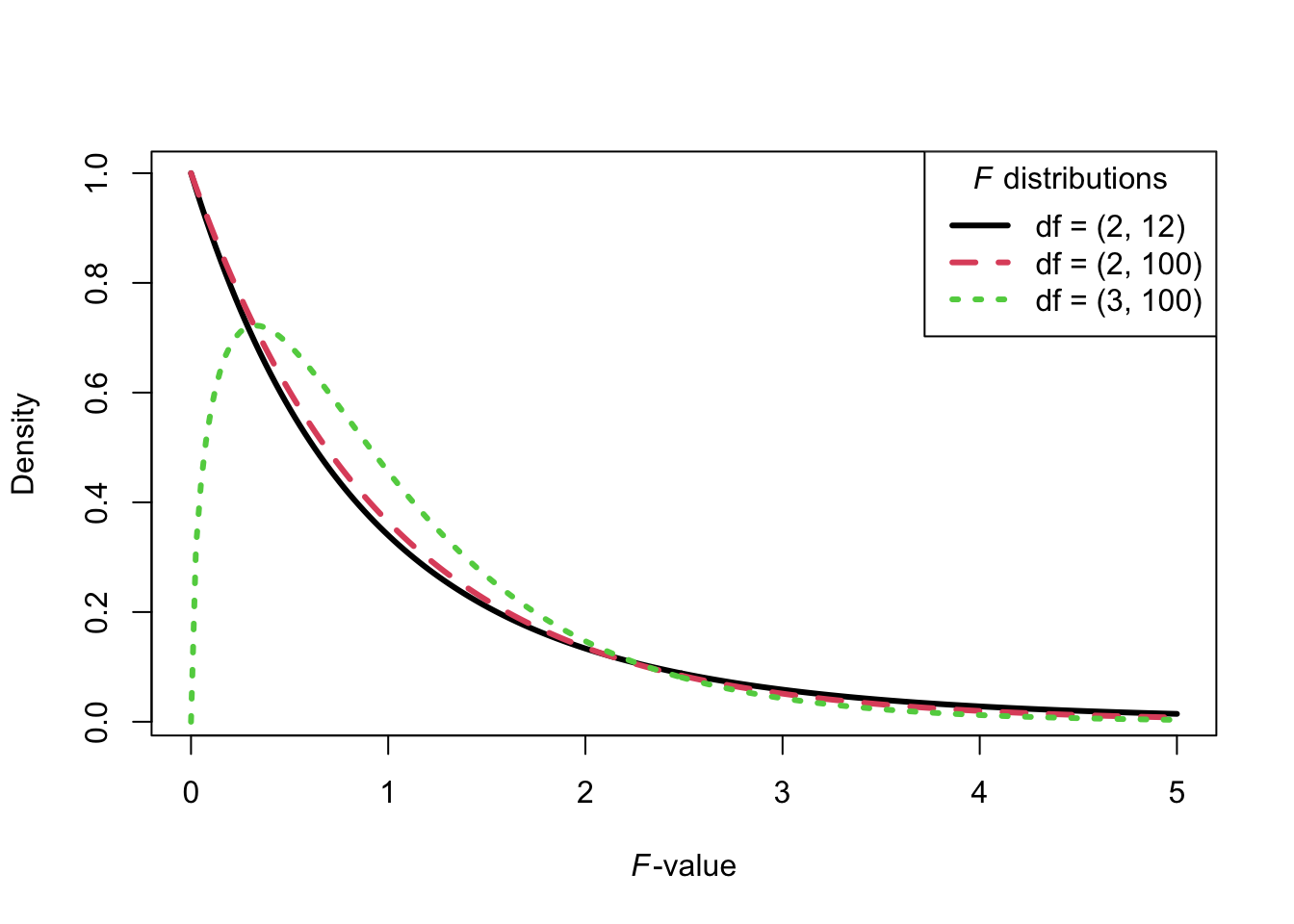
Figure 10.1: Examples of \(F\)-distributions.
Similar to a \(z\)-test (Chapter 7) or a \(t\)-test (Chapter 8), we reject the null hypothesis if the observed value of the \(F\)-ratio (the test statistics) lies in the critical region of the corresponding \(F\)-distribution. Unlike \(z\)-test and \(t\)-test, however, \(F\)-test is a one-sided test, which means that we reject \(H_0\) in favour of \(H_A\) if \(F\) is larger than the 95% quantile (when \(\alpha\) is set at 0.05 level).
For example, the shaded area in Figure 10.2 is the critical region given the significance level \(\alpha\) = 0.05. Its left boundary corresponds to the \(F\) = 2.79, a.k.a. critical \(F\) value. with which we compare our observed \(F\) value. If the observed \(F\) value is larger than the critial \(F\) value, it would fall into the critical region, and we would reject our null hypothesis in favour of the alternative hypothesis. As usual, the \(p\) value is the probability of obtaining an \(F\) value as extreme or more extreme than the one we observed in the current sample.
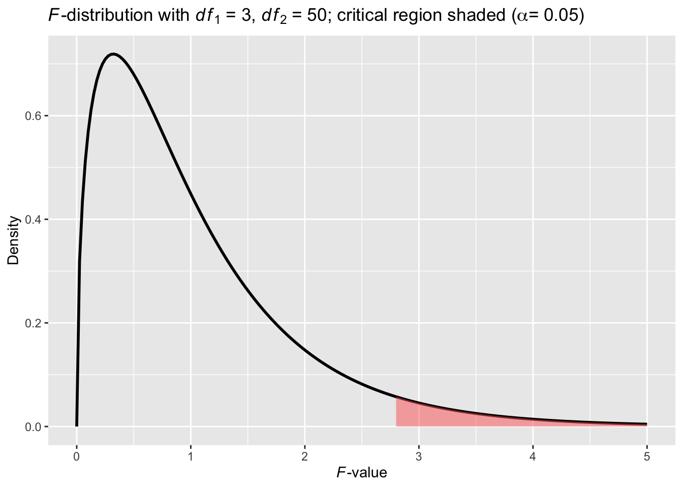
Figure 10.2: A theory-based \(F\)-Distribution
10.1.2 Put it together
To illustrate, let’s fill in Table 10.3 using actual values from the current toy sample data in Table 10.2. I reproduce both of them below in Table 10.4.
|
|
\[ \begin{aligned} &\text{between-treatment variance} = \frac{SS_B}{df_B} = MS_B \\ &= \frac{\sum_{j = 1}^k n_j (\bar{X}_j - \bar{X})^2}{k - 1} \\ &= \frac{5 \cdot (5-3)^2 + 5 \cdot (1-3)^2 + 5 \cdot (3-3)^2}{3-1} \\ &= \frac{20 + 20 + 0}{2} = \frac{40}{2} = 20 \end{aligned} \tag{10.4} \]
\[ \begin{aligned} &\text{within-treatment variance} = \frac{SS_W}{df_W} = MS_W \\ &= \frac{\sum_{i, j} (X_{ij} - \bar{X}_j)^2}{N - k} \\ &= \frac{5 \cdot (3-5)^2 + 5 \cdot(5-5)^2 + \cdots + 5 \cdot (6-5)^2 + \cdots + 5 \cdot (3-3)^2}{15-3} \\ &= \frac{4 + 0 + 4 + 1 + 1 + 1 + 0 + 4 + 0 + 1 + 0 + 1 + 1 + 4 + 0}{12} \\ &= \frac{22}{12} \approx 1.833 \end{aligned} \tag{10.5} \]
\[ F = \frac{MS_B}{MS_W} = 20 \mathbin{/} 1.833 \approx 10.91 \tag{10.6} \]
| Source | Sum of Squares | Degrees of Freedom | Mean Sum of Squares | \(F\) |
|---|---|---|---|---|
| Between | \(SS_B = 40\) | \(df_B = k - 1 = 2\) | \(MS_B = SS_B \mathbin{/} df_B = 20\) | \(MS_B \mathbin{/} MS_W \approx 10.91\) |
| Within | \(SS_W = 22\) | \(df_W = N - k = 12\) | \(MS_W = SS_W \mathbin{/} df_W \approx 1.833\) | |
| Total | \(SS_T = 62\) | \(N - 1 = 14\) |
We can also compare the observed \(F\) value to its corresponding \(F\) distribution.
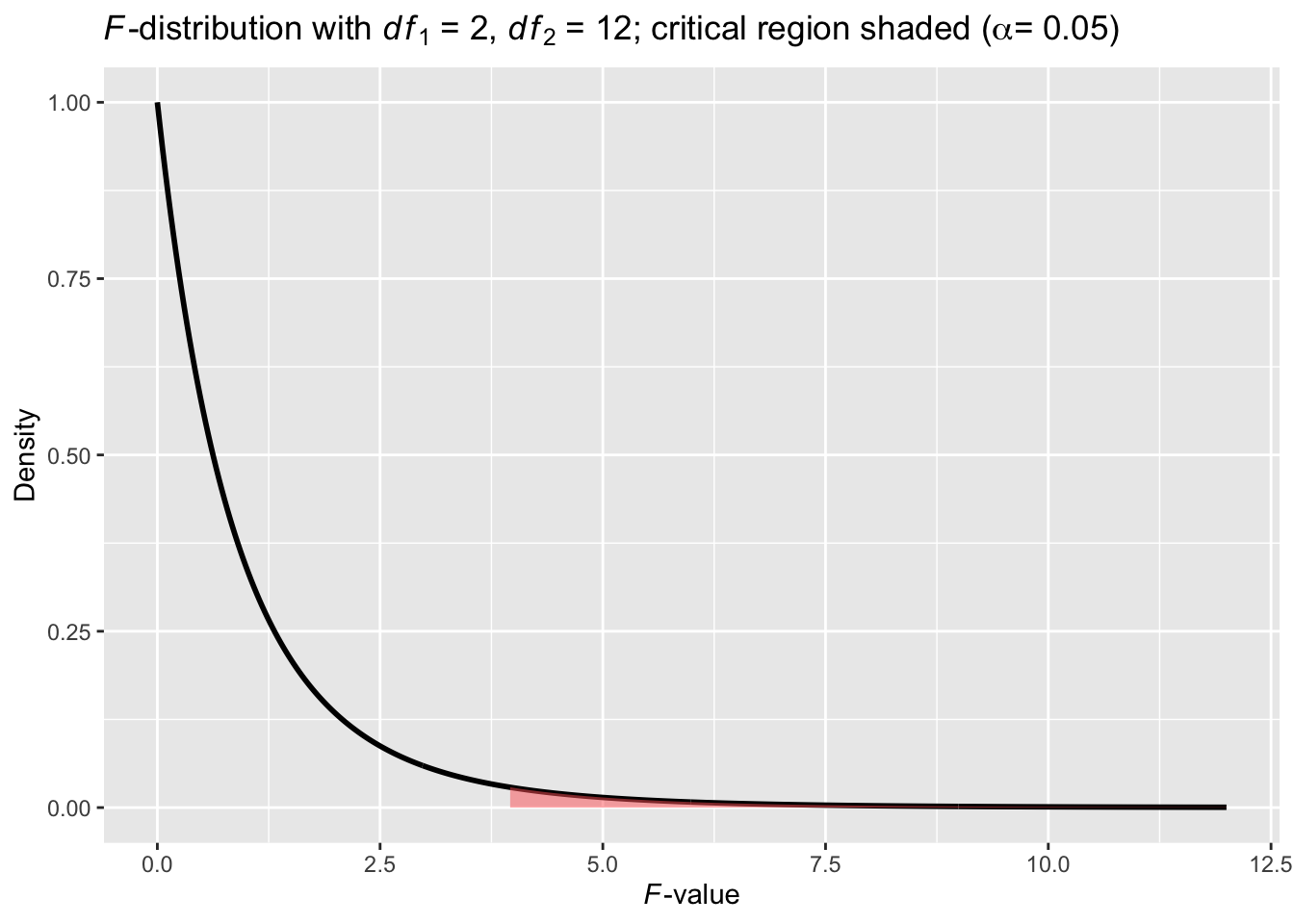
Figure 10.3: A theory-based \(F\)-Distribution for the toy example
Given that the observed \(F_{obs} = 10.91\) falls far into the critical region, we can reject the null hypothesis and conclude that distraction due to cellphone use does seem to affect driving performance adversely.
There are two caveats for the conclusion above. First, a statistically significant \(F\)-value in general only signifies that the population means are not all the same. It does not, however, tells us exactly which pair(s) of means are different. To that end, some post-hoc tests would be required. For this reason, an \(F\)-test is also called an omnibus test (omnibus is literally “for all” in Latin) as it compares all group means simultaneously. Second, whenever the observed \(F\) value is being compared to a theoretical \(F\)-distribution, certain assumptions must be met for the conclusion to be valid. To focus on the logic underlying an ANOVA test, we have omitted the assumptions on purpose in the current toy example. In addition, with a handful of participants in each condition (\(n_1 = n_2 = n_3 = 5\)), it is unlikely that all the assumptions have been met. With a more realistic example next, we will check the assumptions before proceeding to the theory-based methods.
10.2 A realistic example
Problem statement
Sometimes when reading esoteric7 prose we have a hard time comprehending what the author is trying to convey. A student project group decided to replicate part of a seminal 1972 study by Bransford and Johnson on memory encoding (Bransford and Johnson 1972). The study examined college students’ comprehension of following ambiguous prose passage. (Adapted from Ismay)
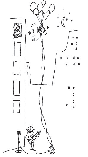
If the balloons popped, the sound wouldn’t be able to carry since everything would be too far away from the correct floor. A closed window would also prevent the sound from carrying, since most buildings tend to be well insulated. Since the whole operation depends on a steady flow of electricity, a break in the middle of the wire would also cause problems. Of course, the fellow could shout, but the human voice is not loud enough to carry that far. An additional problem is that a string could break on the instrument. Then there could be no accompaniment to the message. It is clear that the best situation would involve less distance. Then there would be fewer potential problems. With face to face contact, the least number of things could go wrong.
Did you understand what the passage was describing? Would it help to have some context? The picture that goes along with the passage is shown below:
Before the college students were tested to see whether they understood the passage, they were randomly assigned to one of three groups, and then each group was exposed to the passage under one of the following context conditions:
Students were shown the picture before they heard a recording of the passage (
context before).Students were shown the picture after they heard a recording of the passage (
context after).Students were not shown any picture before or after hearing a recording of the passage (
no context).
Is student comprehension of an ambiguous prose passage affected by viewing a picture designed to aid them in their understanding either before or after? So our research conjecture might be: The population mean comprehension score differs among the three treatments conditions.
Fifty-seven randomly selected students were randomly assigned to be in one of the three groups with nineteen in each group. After hearing the passage under the assigned context condition, they were given a test and their comprehension of the passage was graded on a scale of 1 to 7 with 7 being the highest level of comprehension.
10.2.1 Competing Hypotheses
In words
Null hypothesis: The population mean comprehension scores are the same under all three context conditions (
context before,context after,no context).Alternative hypothesis: At least one of the population mean comprehension scores is different.
In symbols (with annotations)
\(H_0: \mu_{context-before} = \mu_{context-after} = \mu_{no-context}\), where \(\mu\) represents the population mean comprehension score.
\(H_A\): Not all \(\mu\) are equal.
10.2.2 Exploring the sample data
10.2.3 Eyeball the data
Rows: 57
Columns: 2
$ condition     <fct> context after, context after, context after, context af…
$ comprehension <int> 6, 5, 4, 2, 1, 3, 5, 3, 3, 2, 2, 1, 4, 4, 3, 2, 5, 3, 3…
10.2.4 Summary statistics
# Create a template function for descriptives
my_skim <- skimr::skim_with(base = skimr::sfl(n = length, missing = skimr::n_missing),
                     numeric = skimr::sfl(
                                          mean,
                                          sd,
                                          iqr = IQR,
                                          min,
                                          p25 = ~ quantile(., 1/4),
                                          median,
                                          p75 = ~ quantile(., 3/4),
                                          max
                                          ),
                            append = FALSE
) #sfl stands for "skimr function list"
comp %>%
dp$group_by(condition) %>%
my_skim(comprehension) %>%
skimr::yank("numeric") %>%
knitr::kable(
caption = "Summary statistics for comprehension across three conditions",
# control number of digits shown after a decimal point
digits = 2
)| skim_variable | condition | n | missing | mean | sd | iqr | min | p25 | median | p75 | max |
|---|---|---|---|---|---|---|---|---|---|---|---|
| comprehension | context before | 19 | 0 | 4.95 | 1.31 | 2.0 | 2 | 4.0 | 5 | 6 | 7 |
| comprehension | context after | 19 | 0 | 3.21 | 1.40 | 2.0 | 1 | 2.0 | 3 | 4 | 6 |
| comprehension | no context | 19 | 0 | 3.37 | 1.26 | 1.5 | 1 | 2.5 | 3 | 4 | 6 |
The boxplot below also shows the mean for each group highlighted by the red dots.
comp %>%
  gg$ggplot(gg$aes(x = condition, y = comprehension)) +
  gg$geom_boxplot() +
  gg$stat_summary(fun = "mean", geom = "point", color = "red")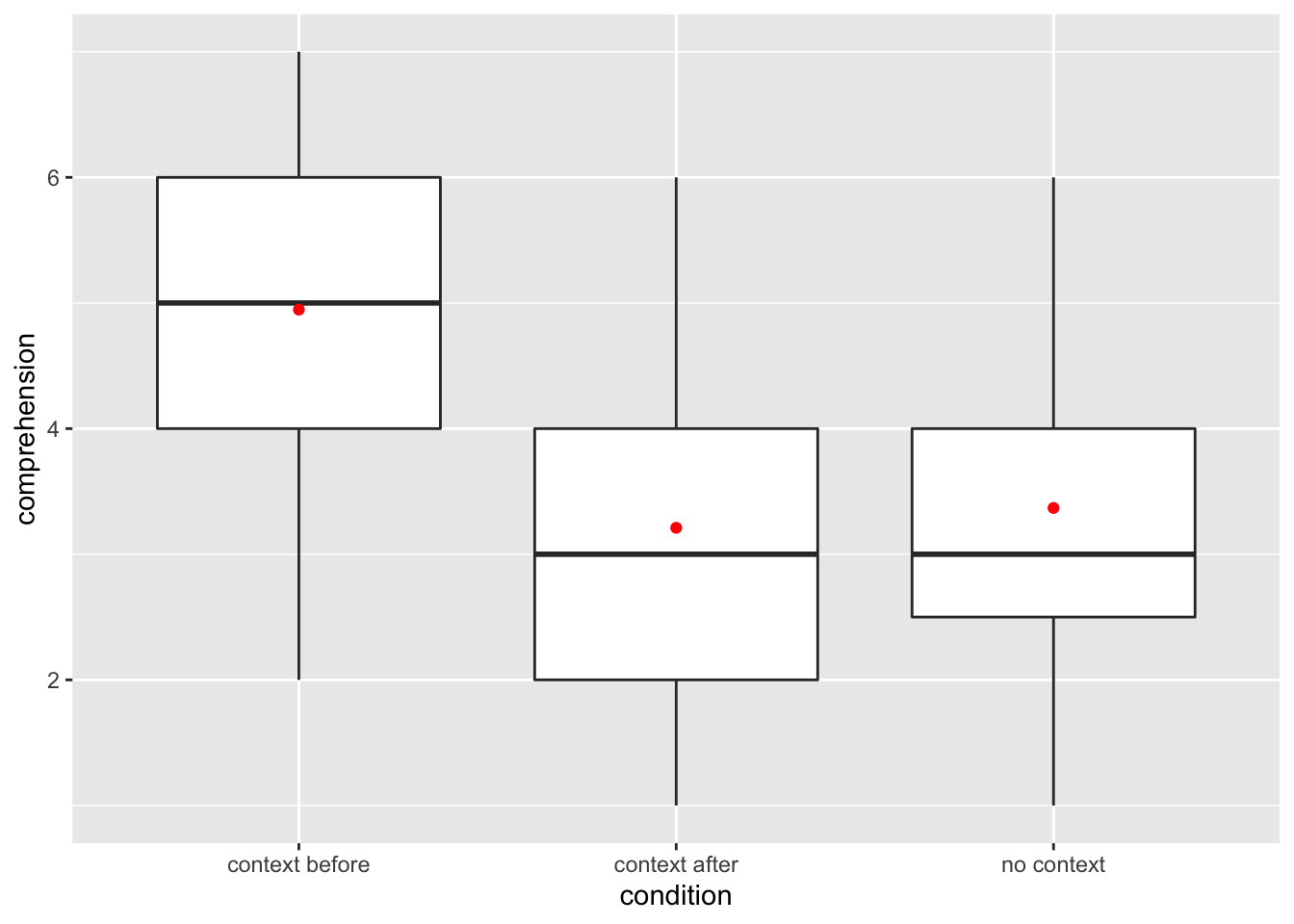
Figure 10.4: Distribution of comprehension scores across three conditions.
Guess about statistical significance
We are testing whether a difference exists in the mean comprehension scores
among the three levels of the explanatory variable — context presence.
Based solely on the boxplot, we have reason to believe that a difference exists,
although the overlapping boxplots of context after and no context conditions
are a bit concerning.
10.2.5 Theory-based methods
Check conditions
Remember that in order to use the theory-based approach, we need to check that the data has met some assumptions. For one-way ANOVA that involves dataset such as the current one, the following assumptions need to be met:
- Independent residuals
- Identically distributed residuals,
These assumptions, independent and identically distributed, are usually abbreviated as i.i.d. The second one can be further broken down to:
- Constant variance
- Normally distributed residuals
All three assumptions involve residual, a concept we have not formally introduced in this book. I have decided to postpone the discussion of this important concept until Chapter 11, because it is much easier to explain what residuals are in the context of regression. And in Chapter 13, you will find out how an ANOVA is nothing but a special case of regression. Until then, I will ask you to take the content in this section at its surface value and try to follow along. We will revisit this section once you have reached Chapter 13.
Independent residuals: The residuals are independent both within and across groups.
This condition is met because students were randomly assigned to be in one of the three groups and were initially randomly selected to be a part of the study. There is no reason to suspect that one person’s response would influence or be influenced by another person’s response.
Constant variance (aka homogeneity of variance): The variance of each condition is about equal from one group to the next.
This is met by observing table 10.6. The
sdvalues are all relatively close and the sample sizes are identical. We can also use the following plot to check this assumption.comp_aov <- aov(comprehension ~ condition, data = comp) plot(comp_aov, which = 1, add.smooth = FALSE) plotrix::draw.ellipse(c(3.2, 3.37, 4.95), c(0, -0.1, -0.3), c(0.05, 0.05, 0.05), c(3, 3, 3), border=1, angle=c(0, 0, 0), lty=3)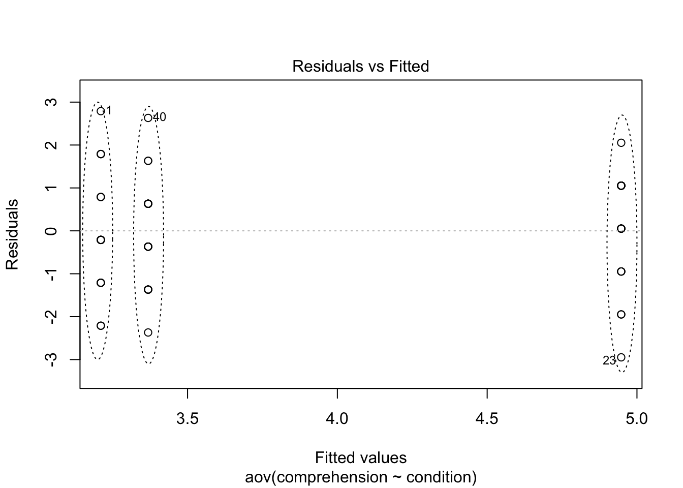
Figure 10.5: The assumption of constant variance is met.
The three collections of data points, each corresponding to one condition, span around the same space, suggesting that constant variance has been met.
Approximately normal: The distribution of the residuals should be normal or the sample sizes should be at least 30 for each group.
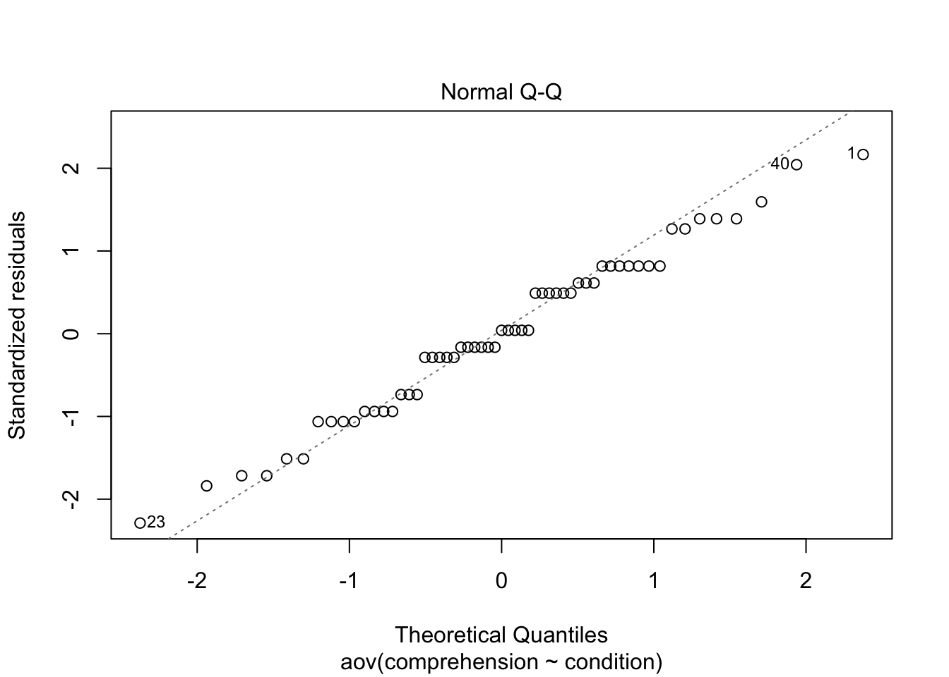
Figure 10.6: The assumption of normality may be in question.
The Q-Q plot shows small deviations from a 1-1 correspondence. Given that the sample sizes for each group is under 30 (\(n = 19\)), we have some reason to doubt the normality assumption here.
Good to know
What if one of more assumptions have been violated?
As you step away from demo data in their ever-perfect condition, and step into the real world where data are anything but perfect, you will often find yourself struggling with violated assumptions. Countless of “xx for dummy” books, bible-like manuals, folklores, and fairytales have been written on how to deal with data that fail to meet certain assumptions. Below is an opinionated summary of what to do when one or more assumptions for a one-way ANOVA have been violated.
Normally distributed residuals. A one-way ANOVA is fairly robust against violations of this assumption. It can tolerate some skewness and kurtosis without inflating the Type I error rate beyond the pre-defined \(\alpha\) level. Between skewness and kurosis, the latter — more peaked or flatter than a standard normal curve — is more important in terms of ensuring valid inferences. If extreme skewness or kurtosis are present, you can apply transformation to the outcome variable, also known as the dependent variable. Some common transformations include square root (\(Y^{\prime} = \sqrt{Y}\)), inverse (\(Y^{\prime} = \frac{1}{Y}\)), and logrithmic (\(Y^{\prime} = \log_e Y\)).
Contant variance (a.k.a. homogeneity). When variance in some groups are visibly larger than in other groups, (e.g., 1.5 times and above, Blanca et al. (2018)) a.k.a. heteroscedasticity, you can use Welch one-way ANOVA test, similar to the Welch two-sample t-test that you have seen in Chapter 8. This test is very similar to the canonical one-way ANOVA test, but with built-in protection against risk of inflated Type I error rate when heteroscedasticity is present. In fact, more recent research has recommended that we use Welch one-way ANOVA test by default, regardless of whether variance is contant or not (Zimmerman 2004). In this chapter, I will demonstrate both canonical and Welch one-way ANOVA on the same data.
In practice, violations of the two aforementioned assumptions often happen in conjunction. For example, applying transformation to the response variable may restore normality as well as equalize group variances. If you have exhausted all remedial measures and the assumptions are still not met, you could use a non-parametric version of one-way ANOVA, such as the Kruskal-Wallis H Test, which does not rely on normality or homogeneity assumptions.
Independent residuals. Violating this assumption is the most serious among the three. Random sampling can guard against such violation to a certain degree. Whenever residuals exhibit some systematic pattern, for example, increase/decrease over time, a different model that can address correlated error terms is in order.
Observed test statistic
Assuming that all three assumptions are met without serious violation, we are ready to apply what we have learned from the previous toy example, and calculate the \(F\)-statistic based on the current sample data. This time, we will leave the tedious calculation to the computer.
Canonical one-way ANOVA
            Df Sum Sq Mean Sq F value Pr(>F)
condition    2  35.05   17.53   10.01 0.0002 ***
Residuals   54  94.53    1.75
---
Signif. codes:  0 '***' 0.001 '**' 0.01 '*' 0.05 '.' 0.1 ' ' 1
Note that we used the aov() function from base R to fit
an ANalysis Of VAriance model to the data.
The summary() function displays the resulting ANOVA table for the model fit.
We see that the \(f_{obs}\) value is 10.01 with \(df_B = k - 1 = 3 - 1 = 2\)
and \(df_W = n_{total} - k = 57 - 3 = 54\).
The \(p\)-value—the probability of observing an \(F(2, 54)\) value of 10.01
or more extreme in our null distribution—is 0.0002.
Welch one-way ANOVA
    One-way analysis of means (not assuming equal variances)

data:  comprehension and condition
F = 9.8552, num df = 2.000, denom df = 35.933, p-value = 0.0003871
Another base R function, oneway.test(),
applies a Welch one-way ANOVA on the same data.
Both the observed \(F\) value and \(p\)-value are comparable
to that obtained using the canonical ANOVA in this case,
likely because the current data met the assumption of constant variance
(Figure 10.5).
Visualize the \(p\) value
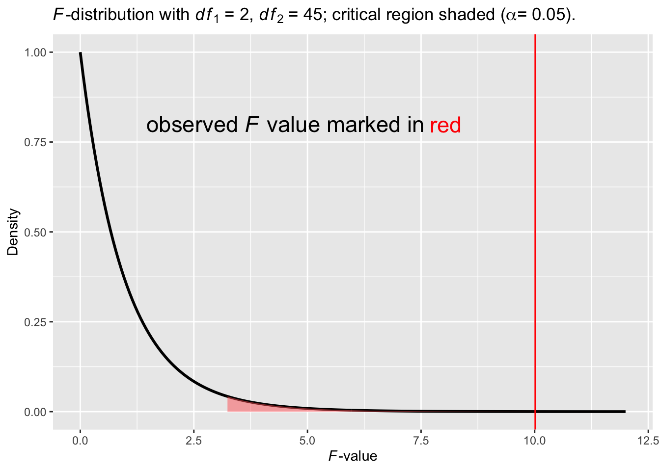
Figure 10.7: An \(F\)-distribution with the observed \(p\)-value
In Figure 10.7, the area shaded in red is the critical region. The red vertical line is where the observed \(F\) value is located (\(F_{obs}\) = 10.01). It falls inside the critical region. The \(p\) value is the area under the curve marked by \(F_{obs}\) and onwards to its right (imagine the x-axis extends to \(+\infty\)). The \(p\) value, 0.0002, is very small, which explains why the area is hardly discernible.
Effect size
In Chapter 9,
we introduced the concept of effect size and demonstrated how to
calculate one for a two-sample \(t\)-test.
Similar to a \(t\)-test, we can also calculate the effect size for an \(F\)-test.
The most common metric of effect sizes for a one-way ANOVA
is the percentage of variance in the outcome variable
accounted for by the treatments, also known as
omega squared
(\(\omega^2\)).
In the current example, for example,
the \(\omega^2\) measures the percentage of variance
in comprehension scores accounted for by context conditions.
Using the terminology we have introduced in Table 10.3, the formula of \(\omega^2\) can be expressed as
\[ \omega^2 = \frac{SS_{between} - df_{between} \cdot MS_{within}}{SS_{between} + SS_{within} + MS_{within}} \tag{10.7} \]
Although we could calculate the effect size \(\omega^2\) for the current example by hand using Equation (10.7), let’s leave the computatation to the computer.
[1] 0.24Interpretation of \(\omega^2\). When/whether the context is provided could account for 24% of the total variance in participants’ comprehension scores.
Good to know
Omega squared, partial omega squared, eta squared, partial eta squared
When you run the function effectsize::omega_squared() above,
you will likely have received a message like the following:
For one-way between subjects designs,
partial omega squared is equvilant to omega squared.
Returning omega squared.
As it turns out, there exists more than one type of effect size when it comes of ANOVA. Eta squared (\(\eta^2\)), partial eta squared (\(\eta_p^2\)), omega squared(\(\omega^2\)), partial omega squared(\(\omega_p^2\)), epsilon squared (\(\epsilon^2\)), cohen’s \(f\), … By definition, an effect size is meant to help researchers compare their results with each other. Having so many different versions of effect size for just one family of tests — ANOVA in this case — defeats the purpose. So why are there so many versions of effect size? And which one should you choose?
Historically, eta squared (\(\eta^2\)) was adopted as effect size for ANOVA test and became popular for its simplicity.
\[ \eta^2 = \frac{SS_{between}}{SS_{total}} \]
However, statisticians soon realized that eta squared is an estimate of effect size based on the sample information, and tends to overestimate the true effect size in the population. To that end, omega squared was proposed as a less biased estimate.
\[ \omega^2 = \frac{df_{between} \times (MS_{between} - MS_{within})}{SS_{total} + MS_{within}} \]
Over time, statisticians realized that both eta squared and omega squared had one serious flaw:
[eta squared and omega squared] cannot easily be compared between studies, because the total variability in a study (\(SS_{total}\)) depends on the design of a study, and increases when additional variables are manipulated (Lakens 2013).
As an alternative, partial eta squared and partial omega squared were recommended on the ground that they would isolate a given variable from other independent variables present in a study. Note that we have only introduced the simplest ANOVA design in the current chapter, in which there is only one indepedent variable. Therefore, the distinction between eta squared and partial eta squared, or between omega squared and partial omega squared, is not relevant.
\[ \eta_p^2 = \frac{SS_{effect}}{SS_{effect} + SS_{error}} \]
\[ \omega_p^2 = \frac{df_{effect} \times (MS_{effect} - MS_{error})} {df_{effect} \times MS_{effect} + (N - df_{effect} \times MS_{error})} \]
Although by no means perfect, partial omega squared \(\omega_p^2\) does seem to stand out as a promising candidate because it corrects for both sample bias and multi-variable bias. However, SPSS, one of the most popular statistical software among social scientists, decided a long time ago that partial eta squared (\(\eta_p^2\)) would be the default effect size for all ANOVA tests conducted using SPSS.
The bottom line is, the effect size is useful/meaningful so long as researchers agree on which effect size to report. Ideally, we as users of statistics — researchers who use statistics but do not specialize on statistics — would want to heed advice offered by statisticians. In reality, however, we often succumb to convenience and habits. When the recommended practice is inconvenient to follow, for example, because the software we are used to have another default setting, we turn a blind eye to the recommendations.
Lakens and colleagues (Lakens 2013; Albers and Lakens 2018) offered a more nuanced comparison of different effect sizes for ANOVA tests and recommended partial omega squared (also see here).
State conclusion
We have sufficient evidence to reject the null hypothesis and conclude that presence of context or a lack thereof affected participants’ comprehension of an esoteric passage (\(F = 10.01\), \(p < .001\), \(\omega^2 = 0.24\)).
Next step
Although ANOVA test is efficient in that it can simultaneously compare multiple means, a statistically significant ombinus \(F\)-test does not offer further insight beyond the fact that some mean is different from others. Now that the null hypothesis has been rejected, we have reasons to believe that among the three treatment groups, at least one of them resulted in comprehension scores different than others. To detect which pair(s) of mean scores are statistically different, we can conduct some post-hoc test. A post-hoc test, as the name suggests, refers to the test conducted after an omnibus ANOVA test.
In this chapter, we will introduce two types of post-hoc tests applicable to one-way ANOVA. The first one, Tukey’s “Honest Significant Differences” method, is essentially several \(t\)-tests, each one comparing a unique pair of means, and controlling the family-wise probability of Type-I error. Similar to the canonical ANOVA method, Tukey’s HSD method assumes contant variance, or homogeneity. The second one, Games-Howell method, is the Welch version of Tukey’s HSD test. Unlike Tukey’s HSD test, Games-Howell method does not require homogeneity of variance, and is especially useful when group sample sizes are unbalanced and/or group variance is visibly different from one group to another.
# A tibble: 3 x 9
  term  group1 group2 null.value estimate conf.low conf.high   p.adj
* <chr> <chr>  <chr>       <dbl>    <dbl>    <dbl>     <dbl>   <dbl>
1 cond… conte… conte…          0   -1.74    -2.77     -0.702 4.84e-4
2 cond… conte… no co…          0   -1.58    -2.61     -0.544 1.55e-3
3 cond… conte… no co…          0    0.158   -0.877     1.19  9.28e-1
# … with 1 more variable: p.adj.signif <chr>
# A tibble: 3 x 8
.y. group1 group2 estimate conf.low conf.high p.adj p.adj.signif
* <chr> <chr> <chr> <dbl> <dbl> <dbl> <dbl> <chr>
1 comprehe… context b… context… -1.74 -2.81 -0.662 9.97e-4 ***
2 comprehe… context b… no cont… -1.58 -2.60 -0.560 2.00e-3 **
3 comprehe… context a… no cont… 0.158 -0.897 1.21 9.29e-1 ns Both tests return highly similar results for the current sample. On average, participants understood the passage better when they saw the context in advance (\(M = 4.95\)), compared to when they saw the context afterwards (\(M = 3.21\)) or did not see the context at all (\(M = 3.37\)). Seeing the context afterwards is as useless as not seeing the context at all (\(p = 0.93\)).
10.3 Conclusion
Thus far, we have walked you through a complete example of ANalysis Of VAriance using theory-based method, including assumptions checking, computing observed \(F\) statistic and \(p\) value, computing effect size, conducting post-hoc tests, and stating conclusion. If this is the first time you have been exposed to the ANOVA technique, you have only discovered the tip of an iceberg known as the ANOVA family. There is still a long way to go before you master this technique. The good news is that learning resources abound when it comes to ANOVA. I will list a few of them at the end of this chapter for you to explore.
Before we leave this chapter behind, as I promised at the beginning, let’s conduct the same analysis using simulation-based methods.
10.3.1 Simulation-based methods
Note that the simulation-based method is not assumption-free. In this case, it still requires that variance be constant and residuals be independent. Assuming that both of these assumptions have been satisfied, let’s now proceed to the next step.
Collecting summary info
Let’s compute the observed \(F\) statistic:
observed_f_statistic <- comp %>%
    infer::specify(comprehension ~ condition) %>%
    infer::calculate(stat = "F")
observed_f_statistic
# A tibble: 1 x 1
stat
<dbl>
1 10.0Hypothesis test using infer verbs
if (!file.exists(here::here("rds", "comp_null_dist.rds"))) {
  null_distribution <- comp %>%
    infer::specify(comprehension ~ condition) %>%
    infer::hypothesize(null = "independence") %>%
    infer::generate(reps = 3000, type = "permute") %>%
    infer::calculate(stat = "F")
  saveRDS(null_distribution, here::here("rds", "comp_null_dist.rds"))
} else {
  null_distribution <- readRDS(here::here("rds", "comp_null_dist.rds"))
}
null_distribution %>%
infer::visualize() +
infer::shade_p_value(observed_f_statistic,
direction = "greater")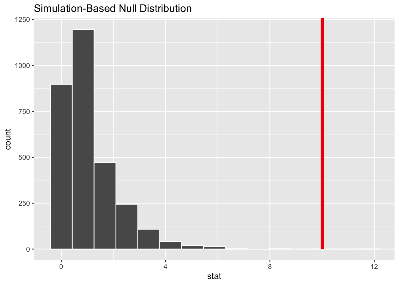
Figure 10.8: Bootstrap distribution for \(F\) test of comprehension scores.
Recall that this is a one-tailed test so we are looking for values that are greater than or equal to the observed \(F\) statistic for the \(p\)-value.
Calculate \(p\)-value
p_value <- null_distribution %>%
    infer::get_p_value(obs_stat = observed_f_statistic,
                                         direction = "greater")
p_value
# A tibble: 1 x 1
p_value
<dbl>
1 0.000333So the \(p\)-value is smaller than the pre-defined \(\alpha\) level and we have enough evidence to reject the null hypothesis at the 5% level. The conclusion would be same as before when we used theory-based methods.
10.3.2 Additional resources
A book by Lukas Meier. This book offers a rigorous treatment of ANOVA. It assumes some algebra and probability background from the reader.
A chapter from a book by David Dalpiaz. A relatively short but still thorough introduction to ANOVA. Similar to Meier’s book, this chapter also assumes some algebra and probability background from the reader.
A book by Danielle Navarro. Similar to the previous two, this book is also heavy on math and probability. However, the author does not assume prior knowledge on probability from the audience. Starting from Chapter 9, the book covers probability all the way to ANOVA in chapter 14.
esoteric | ˌɛsəˈtɛrɪk | adj. intended for or likely to be understood by only a small number of people with a specialized knowledge or interest.↩︎