Chapter 1 Getting Started with Data in R
Before we can start exploring data in R, there are some key concepts to understand first:
- What are R and RStudio?
- How do I code in R?
- What are R packages?
We’ll introduce these concepts in the upcoming Sections 1.1-1.3. If you are already somewhat familiar with these concepts, feel free to skip to Section 1.4 where we’ll introduce our first dataset: all domestic flights departing one of the three main New York City (NYC) airports in 2013.
1.1 What are R and RStudio?
Throughout this book, we will assume that you are using R via RStudio. First time users often confuse the two. At its simplest, R is like a car’s engine while RStudio is like a car’s dashboard as illustrated in Figure 1.1.
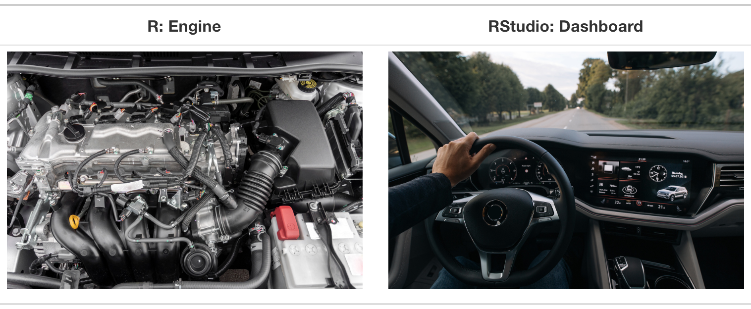
Figure 1.1: Analogy of difference between R and RStudio.
More precisely, R is a programming language that runs computations, while RStudio is an integrated development environment (IDE) that provides an interface by adding many convenient features and tools. So just as the way of having access to a speedometer, rearview mirrors, and a navigation system makes driving much easier, using RStudio’s interface makes using R much easier as well.
1.1.1 Installing R and RStudio
If you have a pre-existing installation of R and/or RStudio, you may skip this part. However, we highly recommend that you upgrade both to the latest version, if they have not been upgraded for a while. Consult Section 1.6.1 if you are not sure how to upgrade.
You will first need to download and install both R and RStudio (Desktop version) on your computer. It is important that you install R first and then install RStudio.
- You must do this first:
Download and install R by going to https://cloud.r-project.org/.
- If you are a Windows user: Click on “Download R for Windows,” then click on “base,” then click on the Download link.
- If you are a macOS user: Click on “Download R for (Mac) OS X,” then under “Latest release:” click on R-X.X.X.pkg, where R-X.X.X is the version number. For example, the latest version of R as of 2020-10-10, was R 4.0.3.
- If you are a Linux user: Click on “Download R for Linux” and choose your distribution for more information on installing R for your setup.
- You must do this second:
Download and install RStudio at
https://www.rstudio.com/products/rstudio/download/.
- Scroll down and look for a big blue button that says
“DOWNLOAD RSTUDIO FOR …,” where
...is your operating system. - Click on the button to start downloading
- Once downloading has completed, double-click it to open, and follow the installation instruction.
- Scroll down and look for a big blue button that says
“DOWNLOAD RSTUDIO FOR …,” where
- Complete this additional step only if you are a macOS user:
Download and install XQuartz.
- Go to https://www.xquartz.org. Under “Quick Download,” click on “XQuartz-2.7.11.dmg.”
- Save the
.dmgfile, double-click it to open, and follow the installation instructions (you may need to restart your computer). - Reminder: you will need to re-install XQuartz when upgrading your macOS to a new major version.
1.1.2 Using R via RStudio
Recall our car analogy from earlier. Much as we don’t drive a car by interacting directly with the engine but rather by interacting with elements on the car’s dashboard, we won’t be using R directly but rather we will use RStudio’s interface. After you install R and RStudio on your computer, you’ll have two new programs (also called applications) you can open. We’ll always work in RStudio and not in the R application. Figure 1.2 shows what icon you should be clicking on your computer.
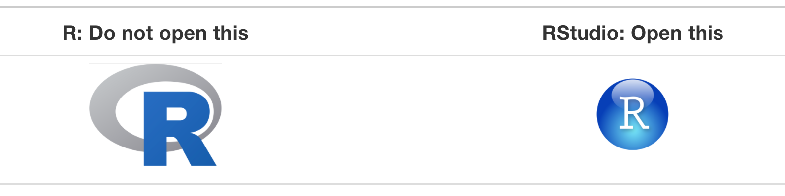
Figure 1.2: Icons of R versus RStudio on your computer.
Unless otherwise specified,
I will be talking about R most of the time during this course,
even though we will be primarily using RStudio.
Here, I use R to refer to the programming language,
rather than the software you have just installed.
I will differentiate R and RStudio
whenever the topic is related to the interface of each application.
After you open RStudio, you should see something similar to Figure 1.3. (Note that slight differences might exist because this snapshot was taken in 2019 and RStudio may have changed their interface since then.)
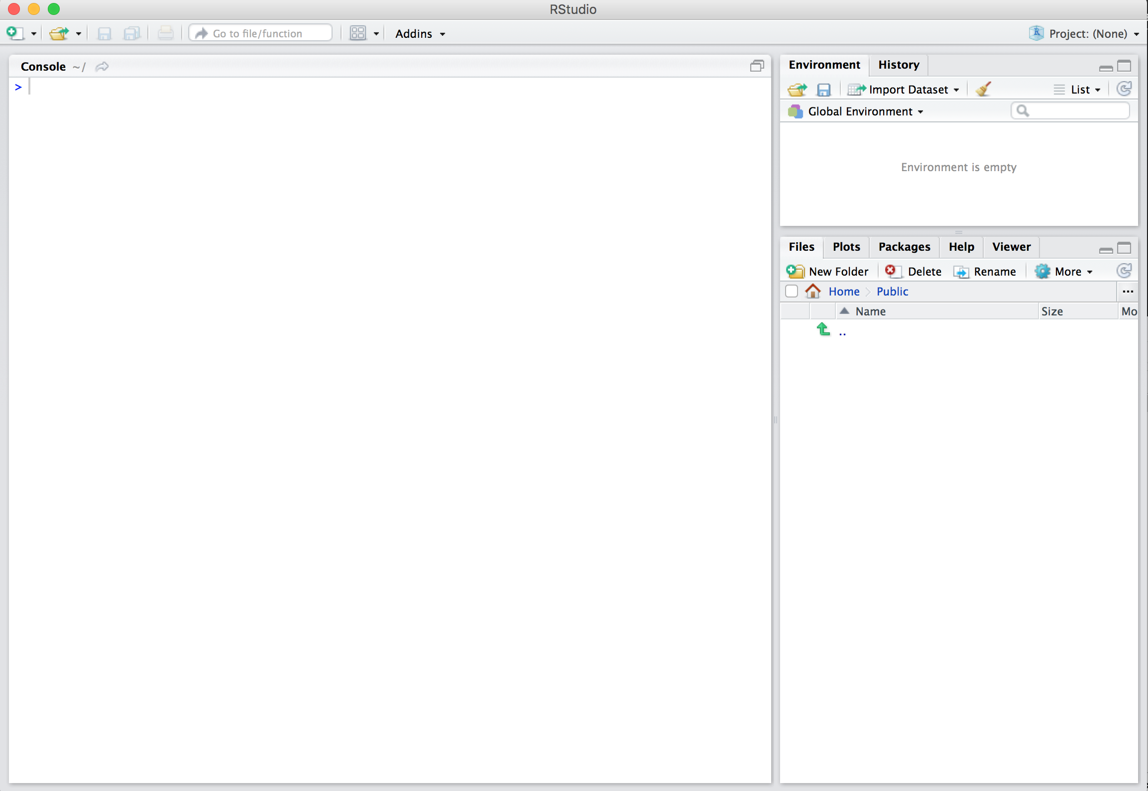
Figure 1.3: RStudio interface to R.
Note the three panes which are three panels dividing the screen: the console pane, the environment pane, and the files pane. Over the course of this chapter, you’ll come to learn what purpose each of these panes serves.
1.1.3 Customize your RStudio
If you had preivously installed R and RStudio and have skipped the section on installation, I encourage you not to skip this part. There might be some recommended setting you have not done despite your familiarity with R and/or RStudio.
- In RStudio, go to Tools >> Global Options, make these changes to the setting as described in Figure 1.4:
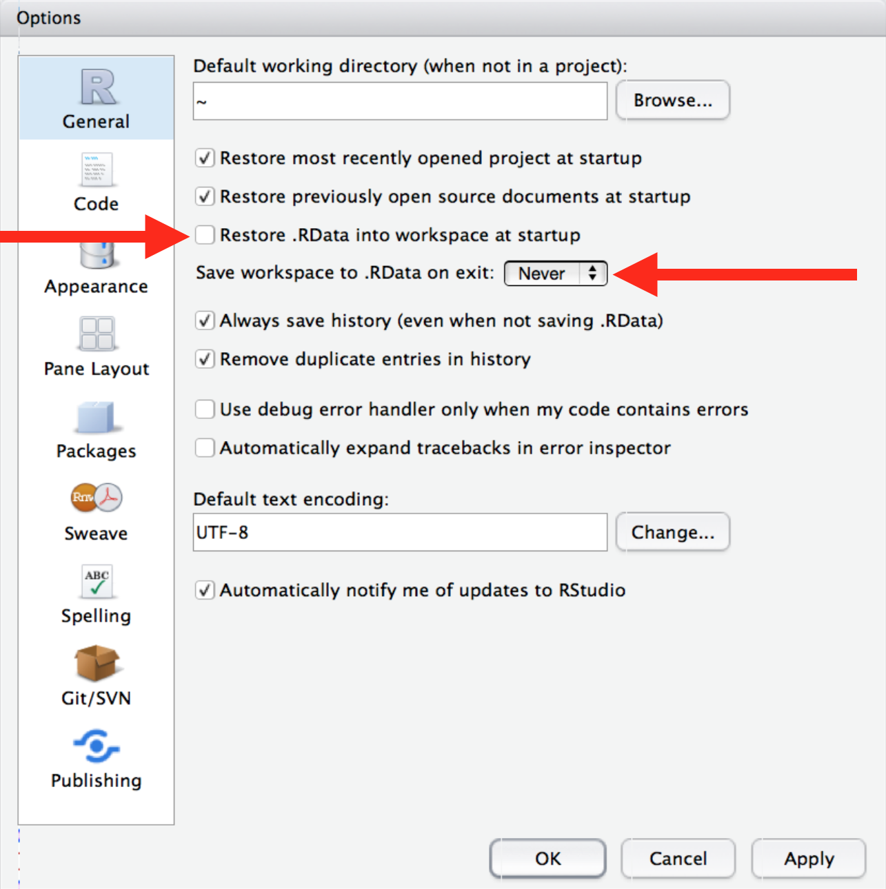
Figure 1.4: Start R with a blank slate, from R for Data Science, chapter 8
[These settings] will cause you some short-term pain, because now when you restart RStudio it will not remember the results of the code that you ran last time. But this short-term pain will save you long-term agony because it forces you to capture all important interactions in your source code. There’s nothing worse than discovering three months after the fact that you’ve only stored the results of an important calculation in your workspace, not the calculation itself in your source code.
- Optionally, you could also adjust the font size
via
Tools >> Global Options >> Appearance >> Editor font size. By default, it is set at 12. I find size 14 easier on my eyes.
1.1.4 Test test test
To make sure you have installed both R and RStudio properly,
type a simple command.
For example, place your cursor in the pane labelled Console,
type x <- 2 + 2, followed by enter or return.
Then type x followed by enter or return.
You should see the value 4 printed to the screen.
If yes, you’ve successfully installed R and RStudio.
1.2 How do I code in R?
The title of this section is mis-leading. No one could answer the question “How to code in R” within a page or two. Instead, what follows is some seeds I want to plant in your head as you begin your coding journey in R. We will revisit all of these concepts applied to various examples as the course unfolds. Before then, I want you to have a preview of them.
As you start using R — the programming language, the first thing to note is that unlike other statistical software programs like Excel, SPSS, or Minitab that provide point-and-click interfaces, R is an interpreted language. This means you have to type in commands written in R code. In other words, you have to code/program in R. Note that we’ll use the terms “coding” and “programming” interchangeably in this book.
While it is not required to be a seasoned coder/computer programmer to use R, there is still a set of basic programming concepts that new R users need to understand. Consequently, while this book is not a book on programming, you will still learn just enough of these basic programming concepts needed to explore and analyze data effectively.
1.2.1 Basic programming concepts and terminology
We now introduce some basic programming concepts and terminology.
Instead of asking you to memorize all these concepts and terminology right now,
we’ll guide you so that you’ll “learn by doing.”
To help you learn, we will always use a different font
to distinguish regular text from computer_code.
The best way to master these topics is, in our opinions,
through deliberate practice
with R and lots of repetition.
- Basics:
- Console pane: where you enter in commands.
- Running code: the act of telling R to perform an act by giving it commands in the console.
- Objects: where values are saved in R. We’ll show you how to assign values to objects and how to display the contents of objects.
- Data types: integers, doubles/numerics, logicals, and characters. Integers are values like -1, 0, 2, 4092. Doubles or numerics are a larger set of values containing both the integers but also fractions and decimal values like -24.932 and 0.8. Logicals are either
TRUEorFALSEwhile characters are text such as “cabbage,” “Hamilton,” “The Wire is the greatest TV show ever,” and “This ramen is delicious.” Note that characters are often denoted with the quotation marks around them.
- Vectors: a series of values. These are created using the
c()function, wherec()stands for “combine” or “concatenate.” For example,c(6, 11, 13, 31, 90, 92)creates a six element series of positive integer values . - Factors: categorical data are commonly represented in R as factors. Categorical data can also be represented as strings. We’ll study this difference as we progress through the book.
- Data frames: rectangular spreadsheets. They are representations of datasets in R where the rows correspond to observations and the columns correspond to variables that describe the observations. We’ll cover data frames later in Section 1.4.
- Conditionals:
- Testing for equality in R using
==(and not=, which is typically used for assignment). For example,2 + 1 == 3compares2 + 1to3and is correct R code, while2 + 1 = 3will return an error. - Boolean algebra:
TRUE/FALSEstatements and mathematical operators such as<(less than),<=(less than or equal), and!=(not equal to). For example,4 + 2 >= 3will returnTRUE, but3 + 5 <= 1will returnFALSE. - Logical operators:
&representing “and” as well as|representing “or.” For example,(2 + 1 == 3) & (2 + 1 == 4)returnsFALSEsince both clauses are notTRUE(only the first clause isTRUE). On the other hand,(2 + 1 == 3) | (2 + 1 == 4)returnsTRUEsince at least one of the two clauses isTRUE.
- Testing for equality in R using
- Functions, also called commands: Functions perform tasks in R. They take in inputs called arguments and return outputs. You can either manually specify a function’s arguments or use the function’s default values.
- For example, the function
seq()in R generates a sequence of numbers. If you just runseq()it will return the value 1. That doesn’t seem very useful! This is because the default arguments are set asseq(from = 1, to = 1). Thus, if you don’t pass in different values forfromandtoto change this behavior, R just assumes all you want is the number 1. You can change the argument values by updating the values after the=sign. If we try outseq(from = 2, to = 5)we get the result2 3 4 5that we might expect. - We’ll work with functions a lot throughout this book and you’ll get lots of practice in understanding their behaviors. To further assist you in understanding when a function is mentioned in the book, we’ll also include the
()after them as we did withseq()above.
- For example, the function
This list is by no means an exhaustive list of all the programming concepts and terminology needed to become a savvy R user; such a list would be so large it wouldn’t be very useful, especially for novices. Rather, we feel this is a minimally viable list of programming concepts and terminology you need to know before getting started. We feel that you can learn the rest as you go. Remember that your mastery of all of these concepts and terminology will build as you practice more and more.
1.2.2 Errors, warnings, and messages
One thing that intimidates new R and RStudio users is how it reports errors, warnings, and messages. R reports errors, warnings, and messages in a glaring red font, which makes it seem like it is scolding you. However, seeing red text in the console is not always bad.
R will show red text in the console pane in three different situations:
- Errors: When the red text is a legitimate error,
it will be prefaced with “Error in…”
and will try to explain what went wrong.
Generally when there’s an error, the code will not run.
For example, we will see in Subsection 1.3.3,
if you receive an error
Error in find.package ... there is no package called ‘import’, it means that the packageimportis not accessible and needs to be installed first. - Warnings: When the red text is a warning, it will be prefaced with “Warning:” and R will try to explain why there’s a warning. Generally your code will still work, but with some caveats. For example, you will see in Chapter 2 if you create a scatterplot based on a dataset where two of the rows of data have missing entries that would be needed to create points in the scatterplot, you will see this warning:
Warning: Removed 2 rows containing missing values (geom_point). R will still produce the scatterplot with all the remaining non-missing values, but it is warning you that two of the points aren’t there. - Messages: When the red text doesn’t start with either “Error” or “Warning,” it’s just a friendly message. You’ll see these messages when you read data saved in spreadsheet files with the
read_csv()function as you’ll see in Chapter 4. These are helpful diagnostic messages and they don’t stop your code from working. Additionally, you’ll see these messages when you install packages usinginstall.packages()as discussed in Subsection 1.3.2.
Remember, when you see red text in the console, don’t panic. It doesn’t necessarily mean anything is wrong. Rather:
- If the text starts with “Error,” figure out what’s causing it. Think of errors as a red traffic light: something is wrong!
- If the text starts with “Warning,” figure out if it’s something to worry about. For instance, if you get a warning about missing values in a scatterplot and you know there are missing values, you’re fine. If that’s surprising, look at your data and see what’s missing. Think of warnings as a yellow traffic light: everything is working fine, but watch out/pay attention.
- Otherwise, the text is just a message. Read it, wave back at R, and thank it for talking to you. Think of messages as a green traffic light: everything is working fine and keep on going!
1.2.3 Tips on learning to code
Learning to code/program is quite similar to learning a foreign language. It can be daunting and frustrating at first. Such frustrations are common and it is normal to feel discouraged as you learn. However, just as with learning a foreign language, if you put in the effort and are not afraid to make mistakes, anybody can learn and improve.
Here are a few useful tips to keep in mind as you learn to program:
- Remember that computers are not actually that smart: You may think your computer or smartphone is “smart,” but really people spent a lot of time and energy designing them to appear “smart.” In reality, you have to tell a computer everything it needs to do. Furthermore, the instructions you give your computer can’t have any mistakes in them, nor can they be ambiguous in any way.
- Take the “copy, paste, and tweak” approach: Especially when you learn your first programming language or you need to understand particularly complicated code, it is often much easier to take existing code that you know works and modify it to suit your ends. This is as opposed to trying to type out the code from scratch. We call this the “copy, paste, and tweak” approach. So early on, we suggest not trying to write code from memory, but rather take existing examples we have provided you, then copy, paste, and tweak them to suit your goals. After you start feeling more confident, you can slowly move away from this approach and write code from scratch. Think of the “copy, paste, and tweak” approach as training wheels for a child learning to ride a bike. After getting comfortable, they won’t need them anymore.
- The best way to learn to code is by doing: Rather than learning to code for its own sake, we find that learning to code goes much smoother when you have a goal in mind or when you are working on a particular project, like analyzing data that you are interested in and that is important to you.
- Practice is key: Just as the only method to improve your foreign language skills is through lots of practice and speaking, the only method to improving your coding skills is through lots of practice. Don’t worry, however, we’ll give you plenty of opportunities to do so!
1.3 What are R packages?
Another point of confusion with many new R users is the idea of an R package. R packages extend the functionality of R by providing additional functions, data, and documentation. They are written by a worldwide community of R users and can be downloaded for free from the internet.
Many R packages
Currently, the number of packages on CRAN, the Comprehensive R Archive Network, is approaching 20,000, and has been growing exponentially. Only four years ago, the number was 10,000. https://blog.revolutionanalytics.com/2017/01/cran-10000.html
For example, among the many packages we will use in this book
are the ggplot2 package (Wickham et al. 2020) for data visualization
in Chapter 2,
the dplyr package (Wickham et al. 2021) for data wrangling in Chapter
3,
the moderndive package (Kim and Ismay 2021) that accompanies this book
,
and the infer package (R-infer?) for “tidy”
and transparent statistical inference in Chapters 6,
7,
and 12.
A good analogy for R packages is they are like apps you can download onto a mobile phone:
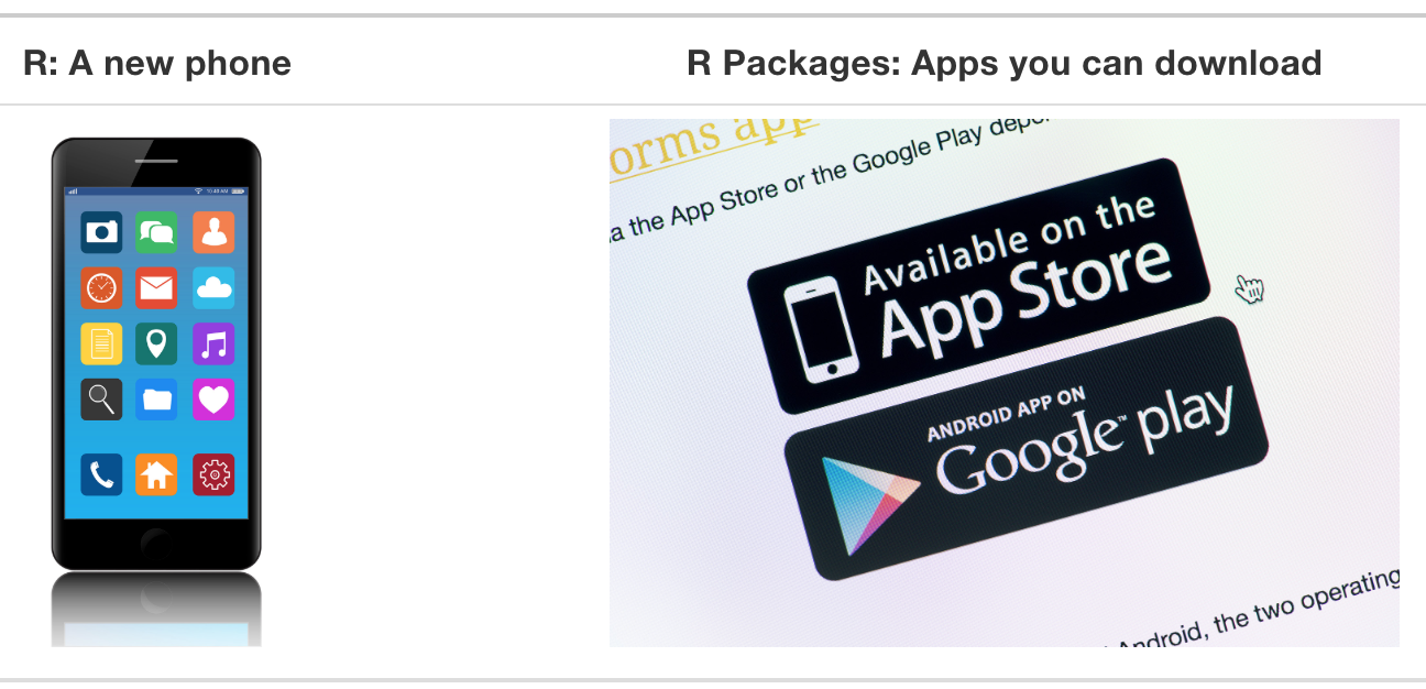
Figure 1.5: Analogy of R versus R packages.
So R is like a new mobile phone: while it has a certain amount of features when you use it for the first time, it doesn’t have everything. R packages are like the apps you can download onto your phone from Apple’s App Store or Android’s Google Play.
Let’s continue this analogy by considering the Instagram app for editing and sharing pictures. Say you have purchased a new phone and you would like to share a photo on Instagram. Since your phone is new and does not include the Instagram app, you need to download and install the app from either the App Store or Google Play. You do this once and you’re set for the time being. You might need to do this again in the future when there is an update to the app. Once Instagram is installed on your phone, you can then proceed to share your photo with your friends and family. assuming you already have an Instagram account set up.
Using an R package is a very similar process. You need to install the package. Although there are some packages already bundled with the base R you just installed from the previous section, most packages are not installed by default when you install R and RStudio. Thus if you want to use such a package for the first time, you need to install it first. Once you’ve installed a package, you likely won’t install it again until you need to update it to a newer version.
1.3.1 Before we install any packages
Having made this much fuss about what packages are, you’d expect that we are going to install some packages next.
I must confess that that is what I have practiced and taught in the past: Set up R and RStudio, install a bunch of packages, and start crunching numbers. Although it is an easier path to take, over the past year or so, I have come to realize that it is not the optimal one. Worse still, it becomes problematic as soon as you finish the course and start tackling real-world data which often are messy and complex. To prepare you for the real world, we must discuss workflow first.
I made this decision, fully aware that this section could be confusing to some of you at first, or even turn away some faint-hearted. Understanding what a workflow is, and setting it up, requires you to be familiar with the basics of R syntax and some programming concepts. However, neither of them is a prerequisite for this course. Therefore, I have to assume that what I am about to explain may seem disconnected or outright nonsense.
I will describe steps for you to follow, and provide rationale for these steps whenever possible. Some of the explanations may still seem nebulous to you, especially if you have not done programming before. Rest assured, by the end of this semester, you will understand them much better. I ask everyone to tolerate some ambiguity at this point. Buckle up. The ride is about to get a bit turbulent.
Setting up a project folder as your first sandbox
During your interaction with RStudio, you will generate different types of files. I recommend that you group these files into project folders. Each folder corresponds to one project. A project could be as simple as a dataset you need to analyze for a course, or as complex as your entire thesis. For the purpose of this course, I suggest that you set up at least two project folders. One for the final project, another as a playground for you to practice various R functions. Let’s start by creating the second project folder, your playground, and name it however you want. For example, go to “Documents” on your computer and create a folder there called “cgsc5101-sandbox.” Think carefully about where this project folder should live. Place it somewhere sensible, so that it will be easy to find in the future.
Good to know
What is in a name?
Do you often have trouble finding a file that you had in mind and end up opening up a bunch of files to see if it is the right one? If so, then you may need to brush up your file-naming skills. It may sound trivial, but naming files is harder than you think. As the late Phil Karlton once put it:
There are only two hard things in Computer Science: cache invalidation and naming things.
https://www.karlton.org/2017/12/naming-things-hard/
I encourage you to check out the following reference for some practical guidance on how to name files (scroll down to see the slides). https://github.com/jennybc/organization-and-naming/tree/master/naming-things
Once this folder has been created, next is to let RStudio know that you want to associate this folder with all the files related to the intended project.
- In RStudio, click the “File” menu button, make sure that the second to last item “Close Project” is greyed out. Otherwise, close the current project that you are in.
- Under the same “File” menu, click “New Project.”
- Click “Existing Directory.”
- Click “Browse,” and select the folder you have just created moments ago, then click “Open.”
- Click the “Create Project” button.
Now, if you look at the folder you have created before,
if it used to be empty, it should have a new file named xxx.Rproj,
where xxx is the name of your folder as well as the project.
To confirm that the project has been set up properly,
- Exist RStudio.
- Double click on the
.Rprojfile.
RStudio should open now, with the the project name displayed on the far right corner of the window.
Execute the following command to add a few more empty subfolders inside the project:
Now you should see these newly added sub-folders inside your project folder.
- data - this will be the subfolder to store raw data files for analysis. These files could be anything from SPSS (.sav) files, Excel / CSV files, or .RDS files. The key idea is that these source data files should be treated as “read-only.” They should be preserved in their original condition to ensure reproducibility.
- scripts - this is where you will store your R scripts and RMarkdown files. This is where you will spend most of your time on.
- results - save all the output from your analysis here, including plots, reports, etc. Treat this folder as disposable. Everything in this folder should be able to be regenerated from your scripts.
Up to this point, you have set up a simple project. There are many ways to set up a project. Look up “R project structure” and take your pick. Here are a few links for you to explore:
Setting up revn
We have completed the first step in our workflow setup.
Next on the agenda is renv.
I will leave out a detailed account of the rationale for now,
and only describe the steps you need to take.
Excute these commands one at a time in the console,
wait while each command takes time to complete.
Lines starting with # are comments.
# install package "remotes"
if (!requireNamespace("remotes")) install.packages("remotes")

# install package "renv"
remotes::install_github("rstudio/renv")

# initialize `renv` for the current project
renv::init()
After successfully executing these three commands, use the RStudio menu itme “Session >> Restart R” to restart R. Alternatively, you can use keyboard shortcut Ctrl+Shift+F10 (Windows and Linux) or Command+Shift+F10 (Mac OS) to restart R.
Inside the console, type .libPaths(),
and confirm that the output looks similar to this:
[1] “/Users/chunyun/Documents/cgsc5101-sandbox/renv/library/R-4.0/…”
[2] ...Presumably, your output will not have “chunyun,” but your own user name, and the “cgsc5101-sandbox” would be replaced with whatever folder name you have used.
If the output looks different, repeat the three commands I have mentioned and try again, or consult Google. If nothing works, book a coaching session with me.
If you get a warning that starts with
“The following required packages are not installed,”
try execute an additional command renv::hydrate(),
followed by renv::snapshot(), to update the state of the project.
Confirm that renv is working properly by typing .libPaths() again
in the console and look for an output as described above.
At this point, you should find an additional file called renv.lock
and a folder renv in your project folder.
Congratulations! You have set up a workflow
that will prove its value as you learn to become a pro.
Now you are ready to install more packages.
Let’s install the ggplot2 package for data visualization.
1.3.2 Package installation
Install ggplot2 by typing install.packages("ggplot2")
in the console pane of RStudio and pressing Return/Enter on your keyboard.
Note you must include the quotation marks around the name of the package.
Much like an app on your phone, you only have to install a package once.
Learning check
(LC1.1)
Repeat the earlier installation steps, but for the dplyr, nycflights13, and knitr packages. This will install the earlier mentioned dplyr package for data wrangling, the nycflights13 package containing data on all domestic flights leaving a NYC airport in 2013, and the knitr package for generating easy-to-read tables in R. We’ll use these packages in the next section.
1.3.3 Package use
What I am about to explain is arguably one of the most controversial topics in the R community. I personally summarize it as “to attach or not to attach.” I spent many hours mulling over which aproach to take for this class. In the end, I decided to take the second, slightly harder one. I believe that you will benefit from this seemingly harder approach in the long run.
Now that you have installed the package ggplot2,
you have gained access to all the functions that come with,
such as geom_point, geom_bar, geom_histogram, to name a few.
To access a function within a package,
you can type PACKAGE::FUNCTION, such as ggplot2::geom_point.
For example, type ?ggplot2::geom_point in the console
and read about the function geom_point().
As you write more codes, the PACKAGE::FUNCTION becomes rather unwieldy.
Why can’t I juse use FUNCTION without the PACKAGE:: part?
You ask.
This is because FUNCTION without PACKAGE:: is ambiguous.
Say there are two packages PKG1 and PKG2,
both have a function FUNC.
When you type FUNC in your code, which one do you want R to summon?
Is there a way to use functions both explicitly and concisely? Yes! I present the solution first and and then explain how it works.
In plain English, what the code above does is to
place all functions from
ggplot2in a self-contained box,assign a new, shorter name –
ggto this box.
Afterwards, we will be able to refer to any function from ggplot2
using the shorthand form gg$FUNC,
such as gg$geom_point.
If you have been following along and trying all the codes introduced here, you may have encountered an error similar to:
Error in find.package ... there is no package called ‘import’when you typed the previous command.
In the solution presented previously,
you used the function from from the import package.
You need to first install import package before you can use its functions.
Now try the gg <- import::from(...) command and it should run successfully.
For those of you who have used R before,
you may be thinking: what about using library() to attach a package?
This is why I said “controversial” at the beginning.
Please allow me to elaborate.
There are two types of R users.
Those that attach packages using library(),
and those that do not attach packages.
Based on my estimate, 99% of R users fall into first category.
Until three months ago, I was also a “attacher”
Now I am one of the 1%.
And if everything goes well, you will join me in the 1% group
by the end of this chapter.
- This is what majority of
Rusers do:
# first approach
install.packages("ggplot2")
library("ggplot2")
ggplot(data = mpg,
       mapping = aes(displ, hwy)) +
geom_point()- This is what I do now and what I recommend that you do:
# second approach
install.packages("ggplot2")
gg <- import::from(ggplot2, .all=T, .into={new.env()})
gg$ggplot(data = mpg,
          mapping = gg$aes(displ, hwy)) +
  gg$geom_point()
At a glance, the first approach seems more convenient.
So why bother using the second one?
Two reasons.
By using library(),
you would be unleashing all functions from every package into the same pool.
In case there are two functions with identical names, say count(),
from two different packages unleashed into the same pool,
only one of them would be accessible via count();
the other one would be “masked”
and only accessible through explicit referencing, PACKAGE::FUNCTION().
Worse still, you will not know ahead of time which one of the pair
is masked.
If you are familiar with python, library(ggplot2) is akin to
from ggplot2 import *,
which has many undesirable consequences
and is strongly discouraged among python users.
The second reason is more pedagogical.
As I mentioned,
I had been using library() since day one until three months ago.
Three months ago, I started thinking about this course
and something my students told me last year suddenly struck me.
There are so many functions in R, and I often have no clue [which packages] these functions belong to.
When I first heard this comment last winter,
I did not take it very seriously and reassured the student that
it was just part of the learning curve, that over time
they would learn the membership of most commonly used R functions.
However, when I started giving more thoughts to this anecdote,
I realized that it might be an unnecessary obstacle to learning R.
Giving up on library() has a series of consequences,
one of which is needing to modify most of the lecture notes
I have developed last year.
It was not an easy task.
But the more I work on it,
the more I am convinced that this is worthwhile.
For example, over the past few days,
on several occasions I have had to look up a function
mentioned in someone’s code
because the function was used without its package explictly referenced.
If I am experiencing this problem and I am relatively familar with R,
how can I expect learners new to R not stumped by it?
To conclude, I will avoid using library() throughout this course,
and explicitly reference each function in association with its package.
There are two exceptions to this rule.
There are some
Rfunctions that come with every clean install ofR, such asinstall.packages(),c(). These functions are often referred to as “base R functions.” When using them, no package reference is required.Apart from the lecture notes, you will be assigned other reading material and exercises. And most of them will use
library()and non-explicit package reference, over which I have very little control. You are encouraged to look up functions whenever you are unsure which packages they belong to.
1.4 Explore your first datasets
Let’s put everything we’ve learned so far into practice and start exploring some real data!
Data comes to us in a variety of formats,
from pictures to text to numbers.
Throughout this book,
we’ll focus on datasets that are saved in “spreadsheet”-type format.
This is probably the most common way data are collected
and saved in many fields.
Remember from Subsection 1.2.1 that
these “spreadsheet”-type datasets are called
data frames in R.
We’ll focus on working with data saved as data frames throughout this book.
The first dataset that we are going to see contains on-time data for all domestic flights departing from one of New York City’s three main airports in 2013: Newark Liberty International (EWR), John F. Kennedy International (JFK), and LaGuardia Airport (LGA).
The following code gives us access to the data, as well as the to some tools so we can interact with the data. Make sure that you run them before proceeding.
# Install xfun so that we can use xfun::pkg_load2
if (!requireNamespace('xfun')) install.packages('xfun')
xf <- loadNamespace('xfun')

cran_primary <- c(
                  "dplyr",
                  "knitr",
                  "nycflights13"
)
cran_secondary <- c(
                    "import"
)

if (length(cran_primary) != 0) xf$pkg_load2(cran_primary)
if (length(cran_secondary) != 0) xf$pkg_load2(cran_secondary)Looks intimidating? Fear not! As the course unfolds, we will unpack codes like these and you will become a master! For now, let me reassure you that the tools are set and the data are ready for inspectation. Let’s proceed!
1.4.1 First impression of a data frame
Let’s begin by exploring the df_flights data frame
and get an idea of its structure.
Run the following code in your console,
either by typing it or by cutting-and-pasting it.
It displays the contents of the df_flights data frame in your console.
Note that depending on the size of your monitor, the output may vary slightly.
# A tibble: 336,776 x 19
    year month   day dep_time sched_dep_time dep_delay arr_time sched_arr_time
   <int> <int> <int>    <int>          <int>     <dbl>    <int>          <int>
 1  2013     1     1      517            515         2      830            819
 2  2013     1     1      533            529         4      850            830
 3  2013     1     1      542            540         2      923            850
 4  2013     1     1      544            545        -1     1004           1022
 5  2013     1     1      554            600        -6      812            837
 6  2013     1     1      554            558        -4      740            728
 7  2013     1     1      555            600        -5      913            854
 8  2013     1     1      557            600        -3      709            723
 9  2013     1     1      557            600        -3      838            846
10  2013     1     1      558            600        -2      753            745
# … with 336,766 more rows, and 11 more variables: arr_delay <dbl>,
#   carrier <chr>, flight <int>, tailnum <chr>, origin <chr>, dest <chr>,
#   air_time <dbl>, distance <dbl>, hour <dbl>, minute <dbl>, time_hour <dttm>
Let’s unpack this output:
A tibble: 336,776 x 19: Atibbleis a specific kind of data frame in R. This particular data frame has336,776rows corresponding to different observations. Here, each observation is a flight.19columns corresponding to 19 variables describing each observation.
year,month,day,dep_time,sched_dep_time,dep_delay, andarr_timeare the different columns, in other words, the different variables of this dataset.- We then have a preview of the first 10 rows of observations corresponding
to the first 10 flights. R is only showing the first 10 rows,
because if it showed all
336,776rows, it would overwhelm your screen. ... with 336,766 more rows, and 11 more variables:indicating to us that 3.368e+05 more rows of data and 11 more variables could not fit in this screen.
This output gives us a nice preview. Let’s look at some different ways to explore data frames.
1.4.2 exploring data frames
There are many ways to get a feel for the data
contained in a data frame such as df_flights.
We present three functions,
all take as their “argument” (their input) the data frame in question.
We also include a fourth method
for exploring one particular column of a data frame:
- using the
View()function, which brings up rstudio’s built-in data viewer. - using the
glimpse()function, which is included in thedplyrpackage. - using the
kable()function, which is included in theknitrpackage. - using the
$“extraction operator,” which is used to view a single variable/column in a data frame.
1. View():
Run View(df_flights)
in your console in rstudio,
either by typing it or cutting-and-pasting it into the console pane.
Explore this data frame in the resulting pop up viewer.
You should get into the habit of viewing any data frames you encounter.
Note the uppercase V in View(). R is case-sensitive,
so you’ll get an error message if you run view(df_flights)
instead of View(df_flights).
learning check
(lc1.2)
what does any one row in this flights dataset refer to?
- data on an airline
- data on a flight
- data on an airport
- data on multiple flights
By running View(df_flights),
we can explore the different variables listed in the columns.
Observe that there are many different types of variables.
Some of the variables like distance, day, and arr_delay
are what we will call quantitative variables.
These variables are numerical in nature.
Other variables here are categorical.
Note that if you look in the leftmost column of the View(df_flights) output,
you will see a column of numbers.
These are the row numbers of the dataset.
If you glance across a row with the same number, say row 5,
you can get an idea of what each row is representing.
This will allow you to identify what object is being described in a given row
by taking note of the values of the columns in that specific row.
This is often called the observational unit. The observational unit in this example is an individual flight departing from new york city in 2013. You can identify the observational unit by determining what “thing” is being measured or described by each of the variables. We’ll talk more about observational units in subsection 1.4.3 on identification and measurement variables.
2. dplyr::glimpse():
The second way we’ll cover to explore a data frame
is using the glimpse() function
included in the dplyr package.
This function provides us with an alternative perspective
for exploring a data frame than the View() function:
Rows: 336,776
Columns: 19
$ year           <int> 2013, 2013, 2013, 2013, 2013, 2013, 2013, 2013, 2013, …
$ month          <int> 1, 1, 1, 1, 1, 1, 1, 1, 1, 1, 1, 1, 1, 1, 1, 1, 1, 1, …
$ day            <int> 1, 1, 1, 1, 1, 1, 1, 1, 1, 1, 1, 1, 1, 1, 1, 1, 1, 1, …
$ dep_time       <int> 517, 533, 542, 544, 554, 554, 555, 557, 557, 558, 558,…
$ sched_dep_time <int> 515, 529, 540, 545, 600, 558, 600, 600, 600, 600, 600,…
$ dep_delay      <dbl> 2, 4, 2, -1, -6, -4, -5, -3, -3, -2, -2, -2, -2, -2, -…
$ arr_time       <int> 830, 850, 923, 1004, 812, 740, 913, 709, 838, 753, 849…
$ sched_arr_time <int> 819, 830, 850, 1022, 837, 728, 854, 723, 846, 745, 851…
$ arr_delay      <dbl> 11, 20, 33, -18, -25, 12, 19, -14, -8, 8, -2, -3, 7, -…
$ carrier        <chr> "UA", "UA", "AA", "B6", "DL", "UA", "B6", "EV", "B6", …
$ flight         <int> 1545, 1714, 1141, 725, 461, 1696, 507, 5708, 79, 301, …
$ tailnum        <chr> "N14228", "N24211", "N619AA", "N804JB", "N668DN", "N39…
$ origin         <chr> "EWR", "LGA", "JFK", "JFK", "LGA", "EWR", "EWR", "LGA"…
$ dest           <chr> "IAH", "IAH", "MIA", "BQN", "ATL", "ORD", "FLL", "IAD"…
$ air_time       <dbl> 227, 227, 160, 183, 116, 150, 158, 53, 140, 138, 149, …
$ distance       <dbl> 1400, 1416, 1089, 1576, 762, 719, 1065, 229, 944, 733,…
$ hour           <dbl> 5, 5, 5, 5, 6, 5, 6, 6, 6, 6, 6, 6, 6, 6, 6, 5, 6, 6, …
$ minute         <dbl> 15, 29, 40, 45, 0, 58, 0, 0, 0, 0, 0, 0, 0, 0, 0, 59, …
$ time_hour      <dttm> 2013-01-01 05:00:00, 2013-01-01 05:00:00, 2013-01-01 …
Observe that dplyr::glimpse() will give you the first few entries
of each variable in a row after the variable name.
In addition, the data type (see subsection 1.2.1)
of the variable is given immediately after each variable’s name inside < >.
Here, int and dbl refer to “integer” and “double,”
which are computer coding terminology for quantitative/numerical variables.
“doubles” take up twice the size to store on a computer compared to integers.
In contrast, chr refers to “character,”
which is computer terminology for text data.
In most forms, text data, such as the carrier or origin of a flight,
are categorical variables.
The time_hour variable is another data type: dttm.
These types of variables represent date and time combinations.
However, we won’t work with dates and times in this book;
we leave this topic for other data science books like
introduction to data science
by Tiffany-Anne Timbers, Melissa Lee, and Trevor Campbell.
or r for data science
by Hadley Wickham.
learning check
(lc1.3) what are some other examples in this dataset of categorical variables? what makes them different than quantitative variables?
3. knitr::kable():
Another way to explore the entirety of a data frame is using the kable()
function from the
knitr package.
Let’s explore the different carrier codes for all the airlines
in our dataset two ways.
Run both of these lines of code in the console:
At first glance, it may not appear that there is much difference in the outputs. However, when using tools for producing reproducible reports such as R Markdown, the latter code produces output that is much more legible and reader-friendly. You’ll see us use this reader-friendly style in many places in the book when we want to print a data frame as a nice table.
4. $ operator
Lastly, the $ operator
allows us to extract and then explore a single variable within a data frame.
For example, run the following in your console
We used the $ operator to extract only the carrier variable
and return it as a vector of length 16.
We’ll only be occasionally exploring data frames using the $ operator,
instead favoring the View() and glimpse() functions.
1.4.3 Identification and measurement variables
There is a subtle difference between the kinds of variables
that you will encounter in data frames.
There are identification variables and measurement variables.
For example, let’s explore another data frame, airports,
using the function we have just used, dplyr::glimpse.
Rows: 1,458
Columns: 8
$ faa   <chr> "04G", "06A", "06C", "06N", "09J", "0A9", "0G6", "0G7", "0P2", …
$ name  <chr> "Lansdowne Airport", "Moton Field Municipal Airport", "Schaumbu…
$ lat   <dbl> 41.13047, 32.46057, 41.98934, 41.43191, 31.07447, 36.37122, 41.…
$ lon   <dbl> -80.61958, -85.68003, -88.10124, -74.39156, -81.42778, -82.1734…
$ alt   <dbl> 1044, 264, 801, 523, 11, 1593, 730, 492, 1000, 108, 409, 875, 1…
$ tz    <dbl> -5, -6, -6, -5, -5, -5, -5, -5, -5, -8, -5, -6, -5, -5, -5, -5,…
$ dst   <chr> "A", "A", "A", "A", "A", "A", "A", "A", "U", "A", "A", "U", "A"…
$ tzone <chr> "America/New_York", "America/Chicago", "America/Chicago", "Amer…
The data frame df_airports contains names, codes, and locations of 1000+
US airports.
The variables faa and name are what we will call identification variables,
variables that uniquely identify each observational unit.
In this case, the identification variables uniquely identify airports.
Such variables are mainly used in practice to uniquely identify
each row in a data frame.
faa gives the unique code provided by the FAA for that airport,
while the name variable gives the longer official name of the airport.
The remaining variables (lat, lon, alt, tz, dst, tzone)
are often called measurement or characteristic variables:
variables that describe properties of each observational unit.
For example,
lat and long describe the latitude and longitude of each airport.
Furthermore, sometimes a single variable might not be enough to uniquely identify each observational unit: combinations of variables might be needed. While it is not an absolute rule, for organizational purposes it is considered good practice to have your identification variables in the leftmost columns of your data frame.
Learning check
(LC1.4)
What properties of each airport do the variables
lat, lon, alt, tz, dst, and tzone
describe in the airports data frame? Take your best guess.
(LC1.5) Provide the names of variables in a data frame with at least three variables where one of them is an identification variable and the other two are not. Further, create your own tidy data frame that matches these conditions.
1.4.4 Help files
R comes with a comprehensive “how-to” manual.
Let’s try to use it:
This is another nice feature of R: its vast collection of help files, which provide documentation for various functions and datasets.
A shorthand for the help function is
by adding a ? before the name of inquiry.
You will then be presented with a page showing the corresponding documentation
if it exists.
Learning check
(LC1.6)
What happens when you type ?flights into the console?
How about ?cars?
1.5 Conclusion
We’ve given you what we feel is a minimally viable set of tools to explore data in R. Does this chapter contain everything you need to know? Absolutely not. To try to include everything in this chapter would make the chapter so large it wouldn’t be useful! As we said earlier, the best way to add to your toolbox is to get into RStudio and run and write code as much as possible.
1.6 Additional resources
If you are new to the world of coding, R, and RStudio and feel you could benefit from a more detailed introduction, we suggest you check out the short book, Getting Used to R, RStudio, and R Markdown (Ismay and Kennedy 2016). It includes screencast recordings that you can follow along and pause as you learn. This book also contains an introduction to R Markdown, a tool used for reproducible research in R.
Figure 1.6: Preview of Getting Used to R, RStudio, and R Markdown.
1.6.1 Upgrade R and/or RStudio
There are many ways to upgrade R and/or RStudio. I will describe one of them here. If you alreays know how to upgrade them, keep doing what you have been doing.
- To upgrade R, find out the current version of R running on your computer. You can do so from within RStudio.
Type R.version.string in the console
and you should see something like this printed out:
[1] “R version 4.0.3 (2020-10-10)”
As of 2021 February, the latest R version is 4.0.4.
If you have an older version installed on your computer,
go to https://cloud.r-project.org and
follow the steps described in 1.1.1 to install the latest version of R.
Restart RStudio and type R.version.string in the console
to confirm the upgrade was successful.
- To upgrade RStudio from within RStudio,
go to
Help > Check for Updatesto install newer version of RStudio (if available). Once both R and RStudio have been upgraded, test by typing some simple command in the console (e.g., 1.1.4).
1.7 What’s to come?
We’re now going to start the “Data Science with tidyverse” portion
of this book in Chapter 2 as shown
in Figure 1.7
with what we feel is the most important tool in a data scientist’s toolbox:
data visualization.
We’ll continue to explore the data included in the nycflights13 package
using the ggplot2 package for data visualization.
You’ll see that data visualization is a powerful tool
to add to your toolbox for data exploration
that provides additional insight
to what the View() and glimpse() functions can provide.
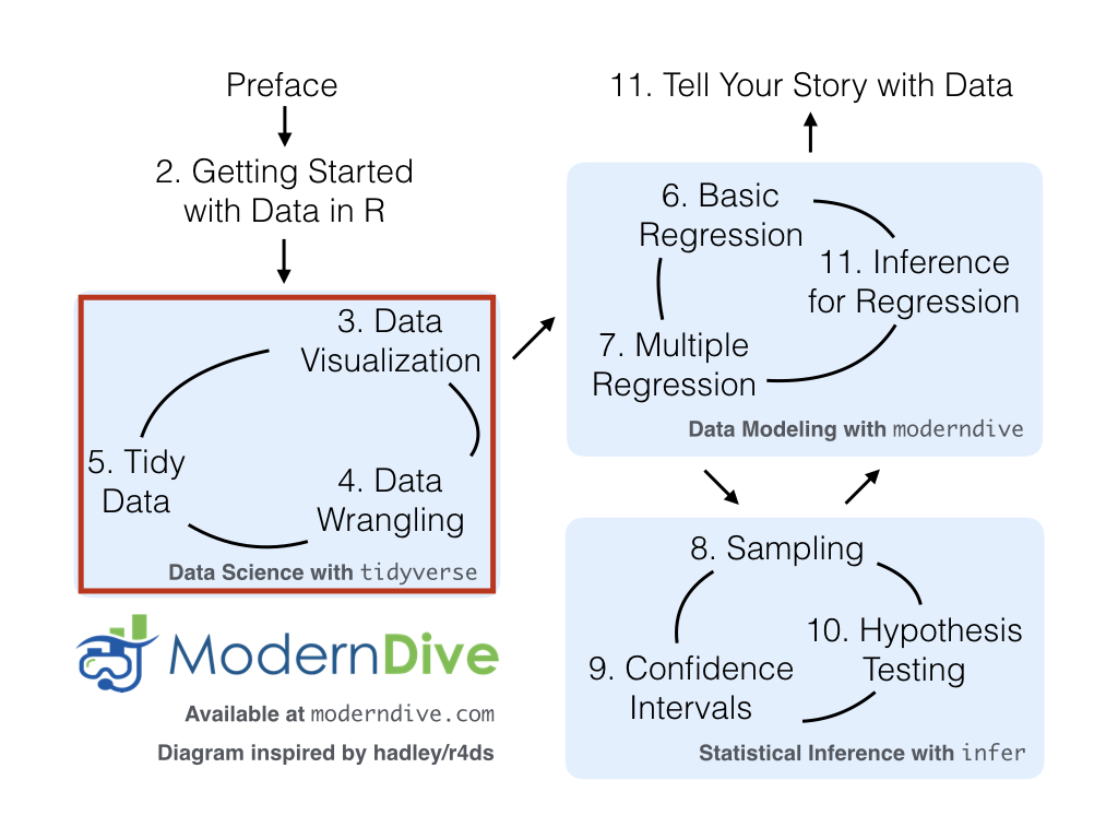
Figure 1.7: ModernDive flowchart - on to Part I!
1.8 Assignment 1
Complete Assignment 1 following instructions in Appendix D.