Chapter 6 Bootstrapping and Confidence Intervals

Let’s start this chapter with an analogy involving fishing. Say you are trying to catch a fish. On the one hand, you could use a spear, while on the other you could use a net.

Recall in Chapter 5 where Cy was trying to estimate the population mean weight $\mu$ of all bananas. Think of the value of $\mu$ as a fish.

On the one hand, she could use the appropriate point estimate/sample statistic to estimate $\mu$, which is the sample mean $\bar{x}$. Based on a sample of 50 bananas, the sample mean was 189. Think of using this value as “fishing with a spear.”

What would “fishing with a net” correspond to? Look at the sampling distribution in Figure 6.1. Between which two values would you say that “most” sample means lie? While this question is somewhat subjective, saying that most sample means lie between 186 and 195 grams would not be unreasonable. Think of this interval as the “net.”

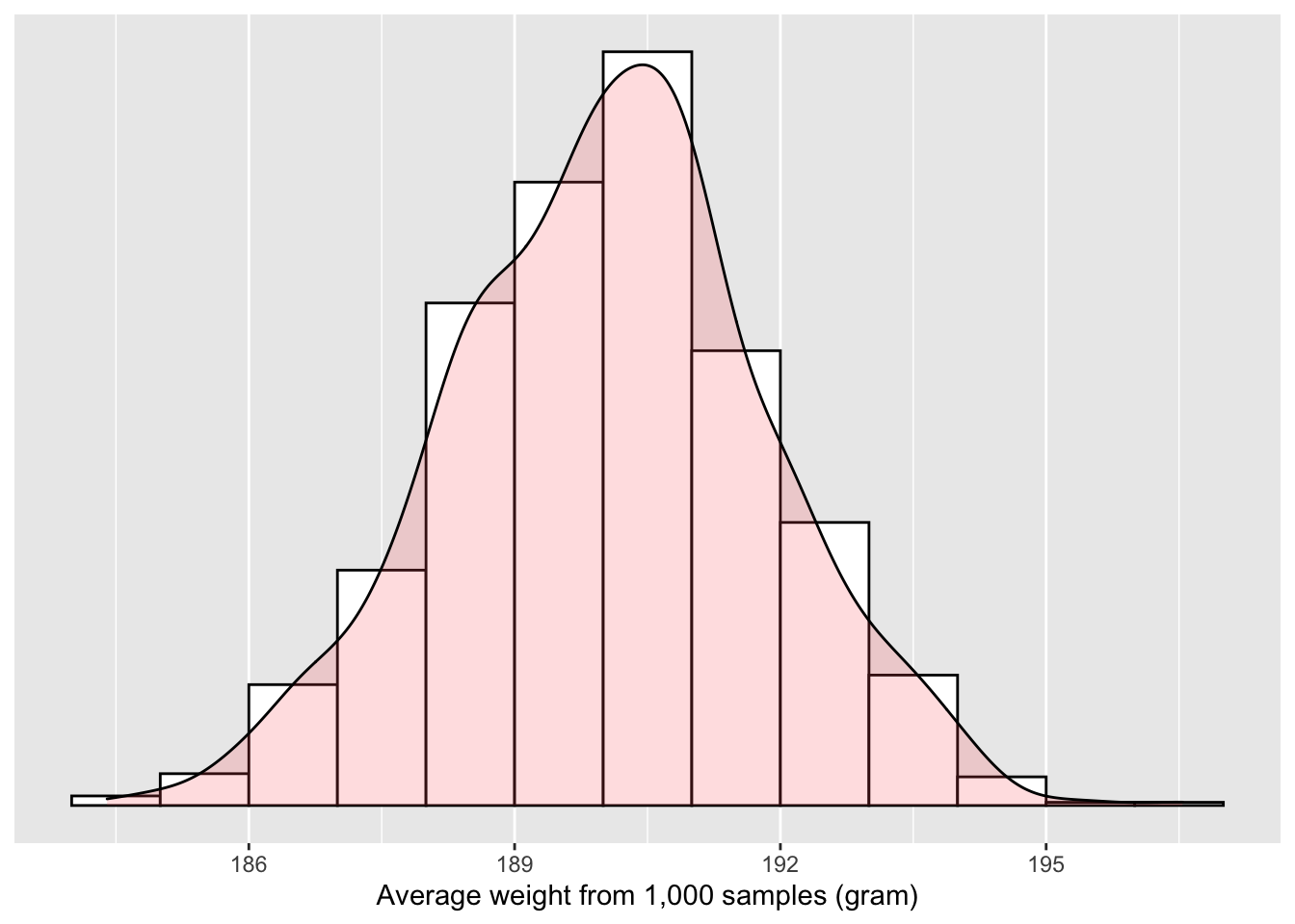
Figure 6.1: Sampling distribution of the mean weight

What we have just illustrated is the concept of a confidence interval. As opposed to a point estimate/sample statistic that estimates the value of an unknown population parameter with a single value, a confidence interval gives what can be interpreted as a range of plausible values. Going back to our analogy, point estimates/sample statistics can be thought of as spears, whereas confidence intervals can be thought of as nets.

Figure 6.2: Analogy of difference between point estimates and confidence intervals.

In this chapter, you will learn:

How to construct confidence intervals for a specific type of population parameter — mean
How to interprete a confidence interval

Once mastered, you will be able to transfer these skills to using confidence intervals for other types of population paramters.

Needed packages

Let’s get ready all the packages we will need for this chapter.

# Install xfun so that I can use xfun::pkg_load2
if (!requireNamespace('xfun')) install.packages('xfun')
xf <- loadNamespace('xfun')

cran_packages <- c(
                  "dplyr", 
                  "ggplot2", 
                  "infer"
)

if (length(cran_packages) != 0) xf$pkg_load2(cran_packages)

gg <- import::from(ggplot2, .all=TRUE, .into={new.env()})
dp <- import::from(dplyr, .all=TRUE, .into={new.env()})

import::from(magrittr, "%>%")
import::from(patchwork, .all=TRUE)

6.1 Constructing a confidence interval

Previously, Cy sampled 1,000 times and plotted the distribution of 1,000 means calculated from those samples. As can be seen from Figure 6.3, a large portion of those means are between the two dashed lines. Recall from Appendix A.4, for a variable that approximates normal distribution, 95% of its values lie within 2 standard deviations¹ above and below the mean.

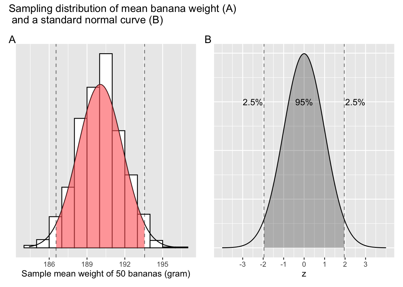
Figure 6.3: Confidence interval based on sampling distributions.

It just so happens that 186.55, the lower bound marked by the dashed line on Figure 6.3 Panel A is two $sd$ below the centre of the distribution, and the upper bound, 193.57, is two $sd$ above the centre. What can you deduce from these pieces of information?

Of the 1,000 means, roughly 95% of them lie between 186.55 and 193.57 grams. This range is commonly knowns as the 95% confidence interval, or CI for short. As statisticians often put it, a banana weighs 190 grams on average, ($CI$ = [186.55, 193.57]).

Next, we learn three different methods of constructing a 95% confidence interval for the estimated mean weight of bananas in the population. Spoiler alert. All three methods lead to similar results for the current example.

6.2 Theory-based approach

Figure 6.3 Panel A is the result of a thought experiment, acted out by our protagonist Cy. In reality, one would rarely collect more than one sample, let alone 1,000 samples! In practice, how do we approximate the sampling distribution in Figure 6.3 without having to go through the trouble of sampling multiple times? Thanks to the Central Limit Theorem, all we need is a sufficiently large sample (n > 30, see Chapter 5.2), at least in the case of estimating populating means.

Using a sample of 50 randomly chosen bananas, we can estimate the centre / peak of the sampling distribution, or the population mean weight of all bananas, a value denoted mathematically by the Greek letter $\mu$. In order to estimate $\mu$, we use the sample mean weight of these 50 bananas as a point estimate, denoted mathematically by $\bar{x}$.

# retrieve a sample of 50 banana weights
banana_sample <- dget("https://raw.githubusercontent.com/chunyunma/baby-modern-dive/master/data/banana_sample.txt")
# compute the sample mean and sample standard deviation
banana_sample %>% 
  dp$summarize(mean = mean(weight), sd = sd(weight))

# A tibble: 1 x 2
   mean      sd
  <dbl>   <dbl>
1 189.3 13.1526

\[ \mu \approx \bar{x} = 189.3 \tag{6.1} \]

In addition, we can estimate the spread of the sampling distribution, commonly denoted by $SE$, using Equation (6.2), which involves the sample standard deviation and sample size.

\[ SE \approx \frac{sd}{\sqrt{n}} = \frac{13.15}{\sqrt{50}} \approx 1.86 \tag{6.2} \]

Thus, the 95% confidence interval for mean weight of banana is:

\[ \begin{aligned} \bar{x} \pm (1.96 \cdot SE_\bar{x}) &= \bar{x} \pm (1.96 \cdot \frac{sd}{\sqrt{n}}) \\ &= 189.3 \pm 1.96 \cdot 1.86 \\ &= 189.3 \pm 3.65 \\ &= [189.3 - 3.65, 189.3 + 3.65] \\ &= [185.65, 192.95] \end{aligned} \tag{6.3} \]

The range is formally called a 95% confidence interval. And the 95% is referred to as the confidence level. We can say that based on our sample, the estimated banana weight is 189.3, with a 95% confidence intevel [185.65, 192.95] (reads “between 185.65 and 192.95”)

This interval centers on the point estimate, $\bar{x} = 189.3$. And it extends to the left and to the right the same magnitude, $1.96 \cdot SE_{\bar{x}}$ . This magtitude is also called the margin of error. The 1.96 multiplier is directly tied to the confidence level, 95%, as explained in Appendix A.4.

The theory-based method only holds if the sampling distribution is normally shaped, so that we can use the 95% rule of thumb about normal distribution discussed in Appendix A.4. When the population parameter in question is a mean, a sufficiently large sample size (n > 30) is all that needed to fulfill the normality requirement, thanks for the Central Limit Theorem. Under the right conditions, the theory-based approach is easy to implement, and requires very little computing power, which is why it has been favoured by researchers in the past. This approach is still widely used today, largely because it is convenient and, above all, familiar to generations of researchers.

In this chapter, we introduce another method for constructing confidence intervals.

6.3 Bootstrapping-based approach

To understand this method, we need to introduce a concept: resampling with replacement.

6.3.1 Resampling once

Step 1: Print out identically sized slips of paper representing the weights of 50 randomly sampled banana.

Step 2: Put the 50 slips of paper into a tuque.

Step 3: Mix the tuque’s contents and draw one slip of paper at random. Record the weight.

Step 4: Place the slip of paper back in the tuque! In another word, RE-place it.

Step 5: Repeat Steps 3 and 4 a total of 49 more times, resulting in 50 recorded weights.

What we just performed was a resampling of the original sample of 50 bananas. Unlike Cy, who sampled repeatedly from the population of bananas, we are mimicking her action by resampling from a single sample of 50 bananas.

Now ask youreself, why did we place our resampled slip of paper back into the tuque in Step 4? Because if we left the slip of paper out of the tuque each time we performed Step 4, we would end up with the same 50 original banana weights! That would make this exercise pointless.

Being more precise with our terminology, we just performed a resampling with replacement from the original sample of 50 bananas. Had we left the paper slip out of the tuque each time we performed Step 4, it would be resampling without replacement.

Let’s compare the weight distribution of the original 50 bananas to that of the re-sampled 50 bananas.

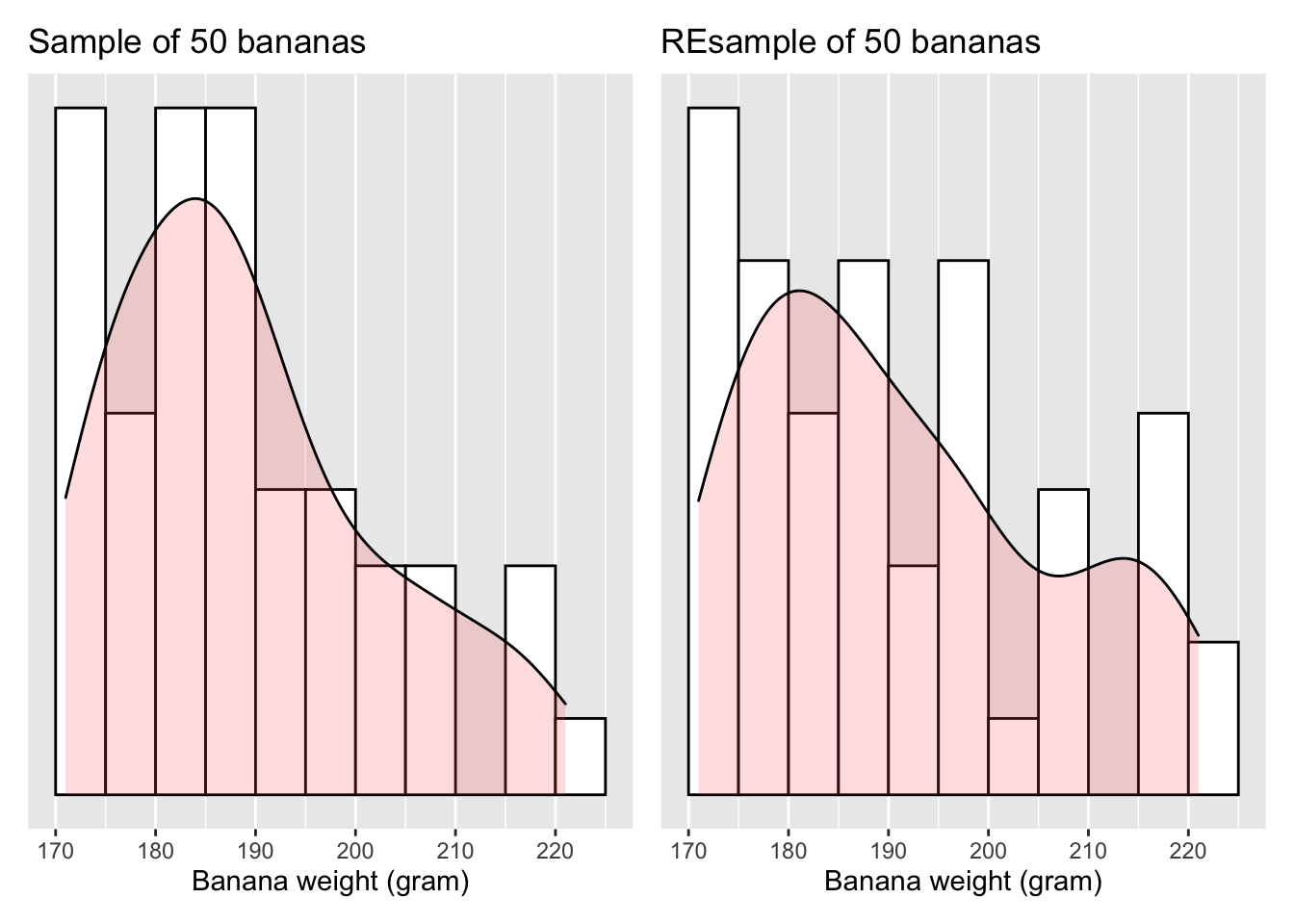
Figure 6.4: Resample and the original sample

Observe in Figure 6.4 that while the general shapes of both distributions of weight are roughly similar, they are not identical. Nor are the mean weights calculated from two distributions.

# retrieve a RE-sample of the original sample
banana_resample <- dget("https://raw.githubusercontent.com/chunyunma/baby-modern-dive/master/data/banana_resample_ch6.txt")
# take a look at the RE-sample
head(banana_resample)

# compute mean of the original sample
m_onesample <- banana_sample %>% 
  dp$summarize(sample_mean = mean(weight))
# compute mean of the RE-sample and compare to that of the original sample
m_oneresample <- banana_resample %>% 
  dp$summarize(resample_mean = mean(weight))
m_onesample
m_oneresample

# A tibble: 1 x 1
  sample_mean
        <dbl>
1       189.3
# A tibble: 1 x 1
  resample_mean
          <dbl>
1         191.5

Resampling from a single sample introduced variation, similar to what Cy has observed by sampling repeatedly from the population (Figure 5.2).

6.3.2 Resampling a thousand times

Resampling from a single sample by following step 1-5 described in Section 6.3.1 does not have obvious advantages compared to sampling from the population. To repeat step 1-5 a thousand times, thereby re-sampling 1,000 times sounds as daunting as what Cy did with the 1,000 samples she collected and measured in Chapter 5. However, although there is no computer algorithm that could sample bananas from the population for Cy, there are reliable algorithms that could resample bananas from a single sample, which makes resampling 1,000 times as trivial as computing a sample mean.

Let’s take one sample and re-sample 1,000 times from it:

# retrieve a sample of 50 banana weights
banana_sample <- dget("https://raw.githubusercontent.com/chunyunma/baby-modern-dive/master/data/banana_sample.txt")
# take a look at the data frame
banana_sample

# A tibble: 50 x 1
   weight
    <dbl>
 1    209
 2    210
 3    186
 4    184
 5    205
 6    182
 7    184
 8    183
 9    175
10    183
# … with 40 more rows

# conduct "sample with replacement" 1,000 times from the original sample
# to produce 1,000 RE-samples 
# Your numbers will be slightly different from mine due to sampling variation
banana_resamples <- banana_sample %>% 
  infer::rep_sample_n(size = 50, replace = T, reps = 1000)
banana_resamples

# A tibble: 50,000 x 2
# Groups:   replicate [1,000]
   replicate weight
       <int>  <dbl>
 1         1    216
 2         1    179
 3         1    198
 4         1    177
 5         1    183
 6         1    182
 7         1    189
 8         1    192
 9         1    189
10         1    221
# … with 49,990 more rows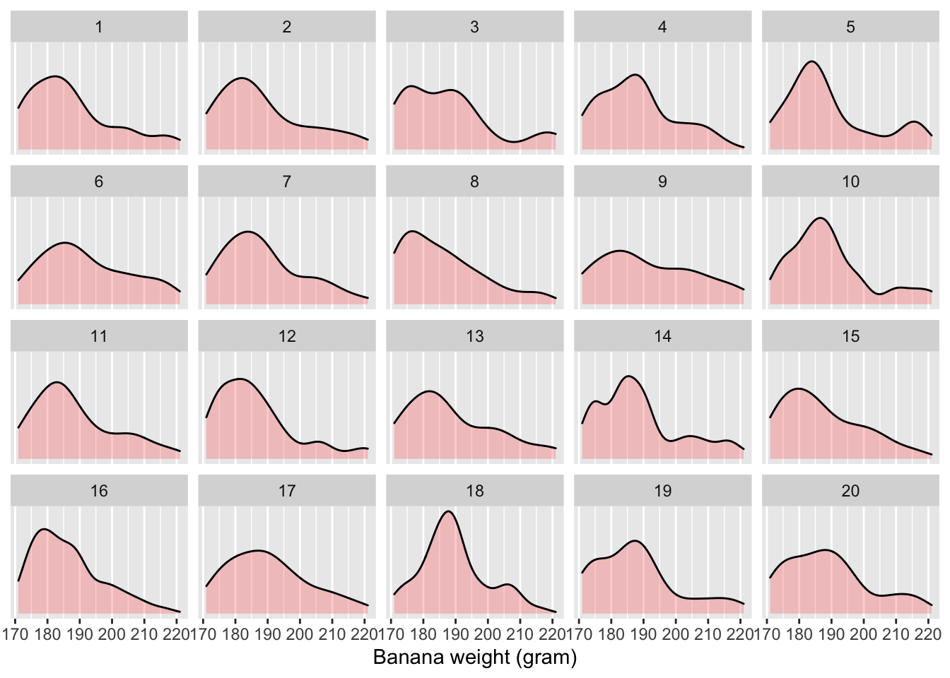

Figure 6.5: Distribution of 50 bananas’ weights in the first 20 REsamples out of 1,000

The resulting banana_resamples data frame has $50 \cdot 1000 = 50,000$ rows corresponding to 1,000 resamples of 50 banana weights. Let’s now compute the resulting 1,000 sample means using the same dplyr::summarize() code as we did in the previous section, but this time adding a group_by(replicate):

resampled_means <- banana_resamples %>% 
  dp$group_by(replicate) %>% 
  dp$summarize(mean_weight = mean(weight))
resampled_means

# A tibble: 1,000 x 2
   replicate mean_weight
 *     <int>       <dbl>
 1         1      187.3 
 2         2      188.28
 3         3      187.88
 4         4      188.06
 5         5      189.4 
 6         6      191.88
 7         7      188.72
 8         8      185.86
 9         9      191.74
10        10      189.4 
# … with 990 more rows

Observe that resampled_means has 1,000 rows, corresponding to the 1,000 resamples. Furthermore, obverse that the values of mean_weight vary. Let’s visualize this variation in Figure 6.6.

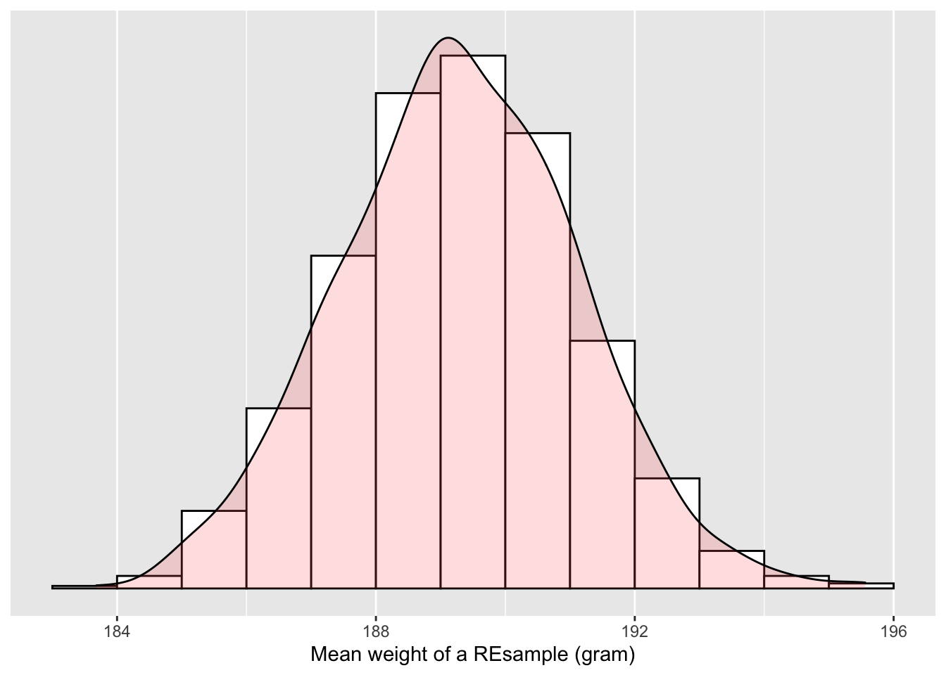
Figure 6.6: Distribution of 1,000 REsample means

What we just demonstrated is the statistical procedure known as bootstrap resampling with replacement. The histrogram in Figure 6.6 is called the bootstrap distribution of the sample mean, constructed by taking 1,000 resamples from a single sample. The bootstrap distribution of the sample mean is an approximation to the sampling distribution, a concept we have discussed in Chapter 5. Like a sampling distribution, a bootstrap distribution allow us to study the effect of sampling variation on our estimates of the population parameter, in this case the mean weight for all bananas. However, unlike Cy in Chapter 5 where she sampled 1,000 times, (something one would never do in practice), bootstrap distributions are constructed by resampling multiple times using a computer algorithm from a single sample: in this case, the 50 original weights of bananas.

The term bootstrapping originates in the expression of “pulling oneself up by their bootstraps,” meaning to “succeed only by one’s own efforts or abilities.”² From a statistical perspective, bootstrapping alludes to succeeding in being able to study the effects of sampling variation on estimates from the “effort” of a single sample. Or more precisely, it refers to constructing an approximation to the sampling distribution using only one sample.

Note in Figure 6.6 that the bell shape is starting to become much more apparent. We now have a general sense for the range of values that the sample mean may take on. Consider: where is this histogram centered? Let’s compute the mean of the 1000 resample means:

resampled_means %>% 
  dp$summarize(mean_of_means = mean(mean_weight))

# A tibble: 1 x 1
  mean_of_means
          <dbl>
1       189.283

The mean of these 1000 means is 189.28 grams, which is quite close to the mean of our original sample of 50 banana weights of 189.3 grams. This is the case since each of the 1,000 resamples is based on the original sample of 50 banana weights.

Congratulations! You’ve just constructed your first bootstrap distribution! In the next section, you’ll see how to use this bootstrap distribution to construct confidence intervals.

6.4 Bootstrapping-based confidence interval

Just as Figure 6.3 provided the information needed to construct a confidence interval — point estimate of mean and standard error of mean, so does Figure 6.6. A 95% confidence interval of sample mean is quite literally locating the lower and upper boundaries on the x-axis of Figure 6.6, such that the values between the said boundaries consists 95% of the whole. We can find the boundaries using either the percentile method, or the standard error method.

6.4.1 Percentile method

To find the middle 95% of values of the bootstrap distribution, we can compute the 2.5th and 97.5th percentiles, which are 185.72 and 192.84, respectively. This is known as the percentile method for constructing confidence intervals.

resampled_means %>% 
  dp$summarize(
               ci_lower = quantile(mean_weight, 2.5/100), 
               ci_upper = quantile(mean_weight, 97.5/100)
  )

# A tibble: 1 x 2
  ci_lower ci_upper
     <dbl>    <dbl>
1  185.719  192.842

Let’s mark both percentitles on the bootstrap distribution in Figure 6.7. About 95% of the mean_weight variable values in resampled_means fall between 185.72 and 192.84, with the remaining 5% of the values fall on either side outside of the boundaries.

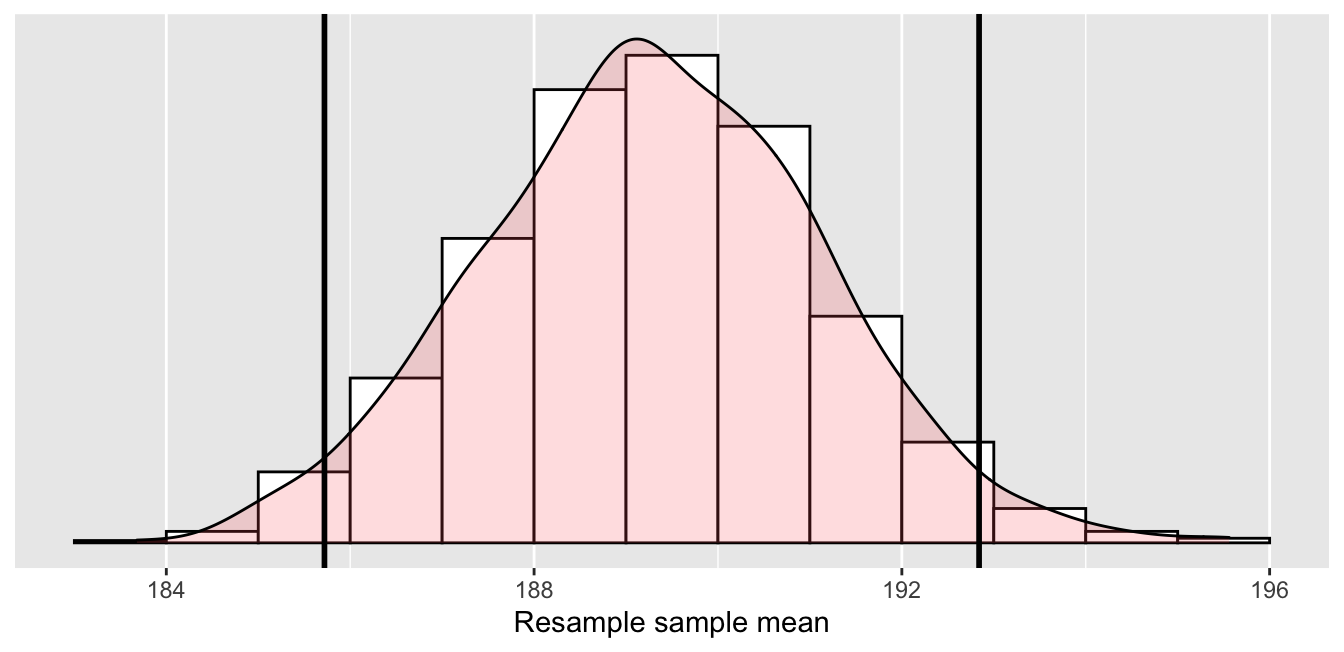
Figure 6.7: Percentile method 95% confidence interval. Interval endpoints marked by vertical lines.

6.4.2 Standard error method

Recall in Appendix A.4, we saw that if a numerical variable follows a normal distribution, or, in other words, the histogram of this variable is bell-shaped, then roughly 95% of values fall between $\pm$ 1.96 standard deviations of the mean. Given that our bootstrap distribution based on 1000 resamples with replacement in Figure 6.6 is normally shaped, let’s use this fact about normal distributions to construct a confidence interval in a different way.

First, recall the bootstrap distribution has a mean equal to mean_of_means = 189.28 grams. Second, let’s compute the standard deviation of the bootstrap distribution using the values of mean_weight in the resampled_means data frame:

resampled_means %>% 
  dp$summarize(SE = sd(mean_weight))

# A tibble: 1 x 1
       SE
    <dbl>
1 1.83166

What is this value? Recall that the bootstrap distribution is an approximation to the sampling distribution. Recall also that the standard deviation of a sampling distribution has a special name: the standard error. Putting these two facts together, we can say that 1.83 is an approximation of $SE_{\bar{x}}$, i.e., the standard error of $\bar{x}$.

Thus, using our 95% rule of thumb about normal distributions from Appendix A.4, we can use the following formula to determine the lower and upper endpoints of a 95% confidence interval for $\mu$:

\[ \begin{aligned} \bar{x} \pm (1.96 \cdot SE) &= (\bar{x} - 1.96 \cdot SE, \bar{x} + 1.96 \cdot SE) \\ &= [189.28 - 1.96 \cdot 1.83, 189.28 + 1.96 \cdot 1.83] \\ &= [185.69, 192.87] \end{aligned} \tag{6.4} \]

Let’s now add the SE method confidence interval with dashed lines in Figure 6.8.

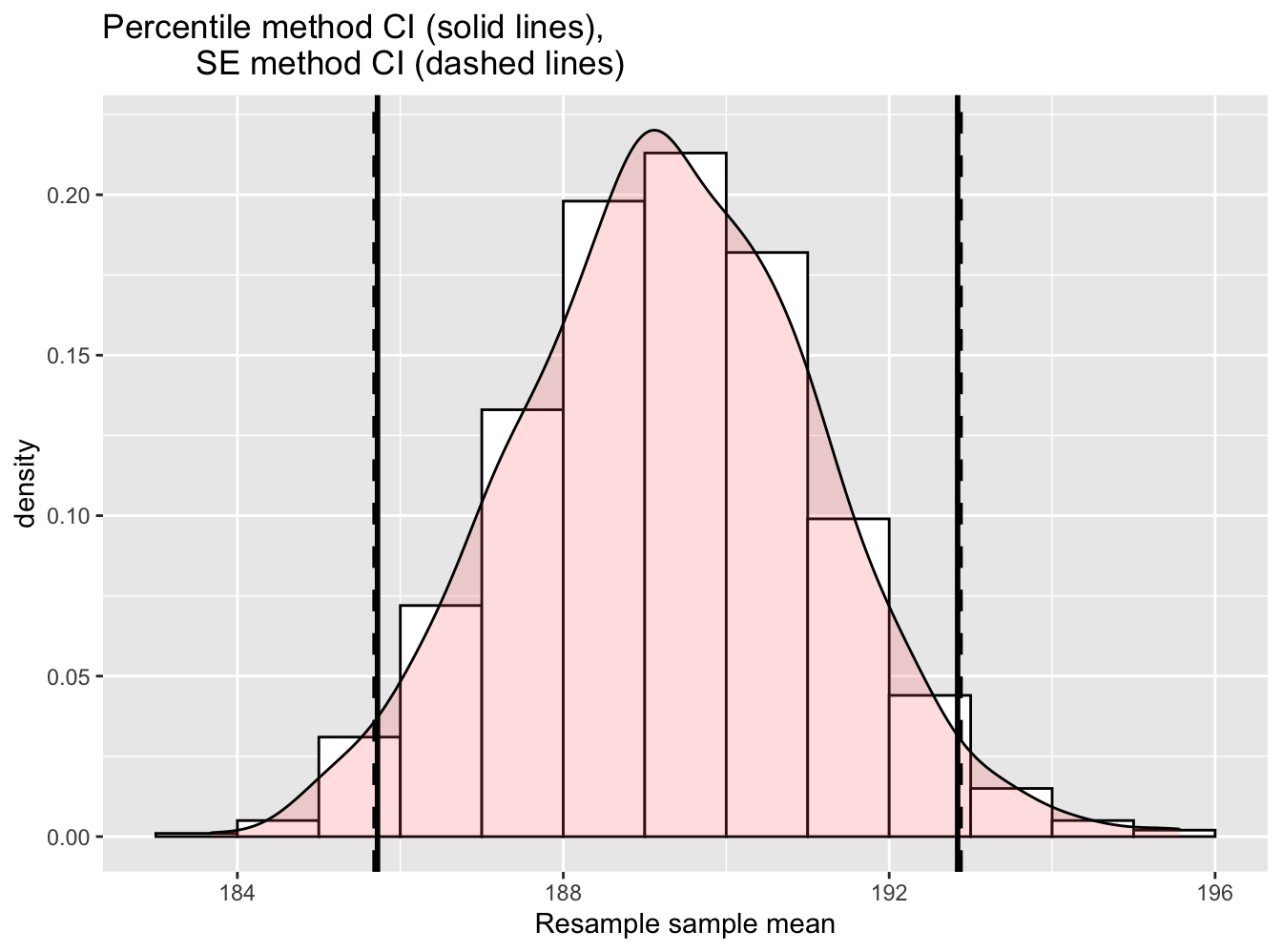
Figure 6.8: Comparing two 95% confidence interval methods.

We see that both methods produce nearly identical 95% confidence intervals for $\mu$ with the percentile method yielding $[185.72, 192.84]$ while the standard error method produces $[185.69, 192.87]$.

6.5 Recap

So far, we have introduced three methods of constructing confidence intervals for the same population parameter. How do they compare to each other?

Table 6.1: Confidence intervals constructed using three methods
Type	lower	upper	Width	Formula	Note
Theroy	185.654	192.946	7.291	$\bar{x}\pm\frac{sd}{\sqrt{n}}$	Requires sampling distribution normality
SE	185.690	192.870	7.180	mean(means) $\pm$ sd(means)	Requires computing power & bootstrap distribution normality
Percentile	185.720	192.840	7.120	[quantile(means, 2.5/100), quantile(means, 97.5/100]	Requires computing power

Theory-based methods have been used in the past because we did not have the computing power to perform simulation-based methods such as bootstrapping. Although convenient, theory-based methods fall short where we cannot estimate sampling distributions from sample statistics. Both Percentile and SE methods are based on bootstrap distribution. The SE methods are applicable when the bootstrap distribution is roughly normally shaped. The Percentile method is the most flexible among the three. It also works when we cannot estimate sampling distributions from sample statistics and/or the bootstrap distribution is not normally shaped.

6.6 Interpreting confidence intervals

Now that we’ve shown you three methods of how to construct confidence intervals using a sample drawn from a population, let’s now focus on how to interpret their effectiveness. The effectiveness of a confidence interval is judged by whether or not it contains the true value of the population parameter. Recall the fishing analogy we introduced at the beginning of this chapter, this is like asking, “Did our net capture the fish?”

So, for example, does our percentile-based confidence interval of [185.72, 192.84] capture" the true mean weight of all bananas? Normally, we will never be able to tell, because we don’t know what the true value of $\mu$ is. After all, we are sampling to estimate it! However, it should not come as a surprise that the “population of bananas” from which Cy drew her numerous samples was simulated by me. Using a special algorithm, I created 100,000 plausible numbers representing the weight of 100,000 bananas. The numbers are stored in the data frame banana_pop.

banana_pop <- dget("https://raw.githubusercontent.com/chunyunma/baby-modern-dive/master/data/banana_pop.txt")
tibble::glimpse(banana_pop)

Rows: 100,000
Columns: 1
$ weight <dbl> 177, 198, 176, 203, 171, 204, 186, 186, 204, 189, 179, 209, 17…

From those numbers, I drew samples such as banana_sample.

banana_sample

# A tibble: 50 x 1
   weight
    <dbl>
 1    209
 2    210
 3    186
 4    184
 5    205
 6    182
 7    184
 8    183
 9    175
10    183
# … with 40 more rows

Although the numbers are fictional, they bear important information that reflects the reality. Let’s calculate (not estimate) the true mean weight of bananas $\mu$ in the simulated population and find out whether or not a confidence interval “captured” this value.

banana_pop %>% 
  dp$summarise(pop_mean = mean(weight))

# A tibble: 1 x 1
  pop_mean
     <dbl>
1  190.122

Now we know that the population mean weight $\mu$ is 190.12 grams. Let’s now compare the confidence interval of mean we have constructured earlier to the true population mean. We will then see if the confidence interval has “captured” the true value of $\mu$.

6.6.1 Did the net capture the fish?

Before we reveal the answer, let’s quickly review the process of how we get here.

An unbiased sample of bananas was randomly chosen.
A bootstrap distribution (which approximates the sampling distribution) was constructed by REsampling multiple times from the said sample.
A confidence interval was constructed using the bootstrap distribution.
The confidencee interval was compared to the true value of the population parameter.

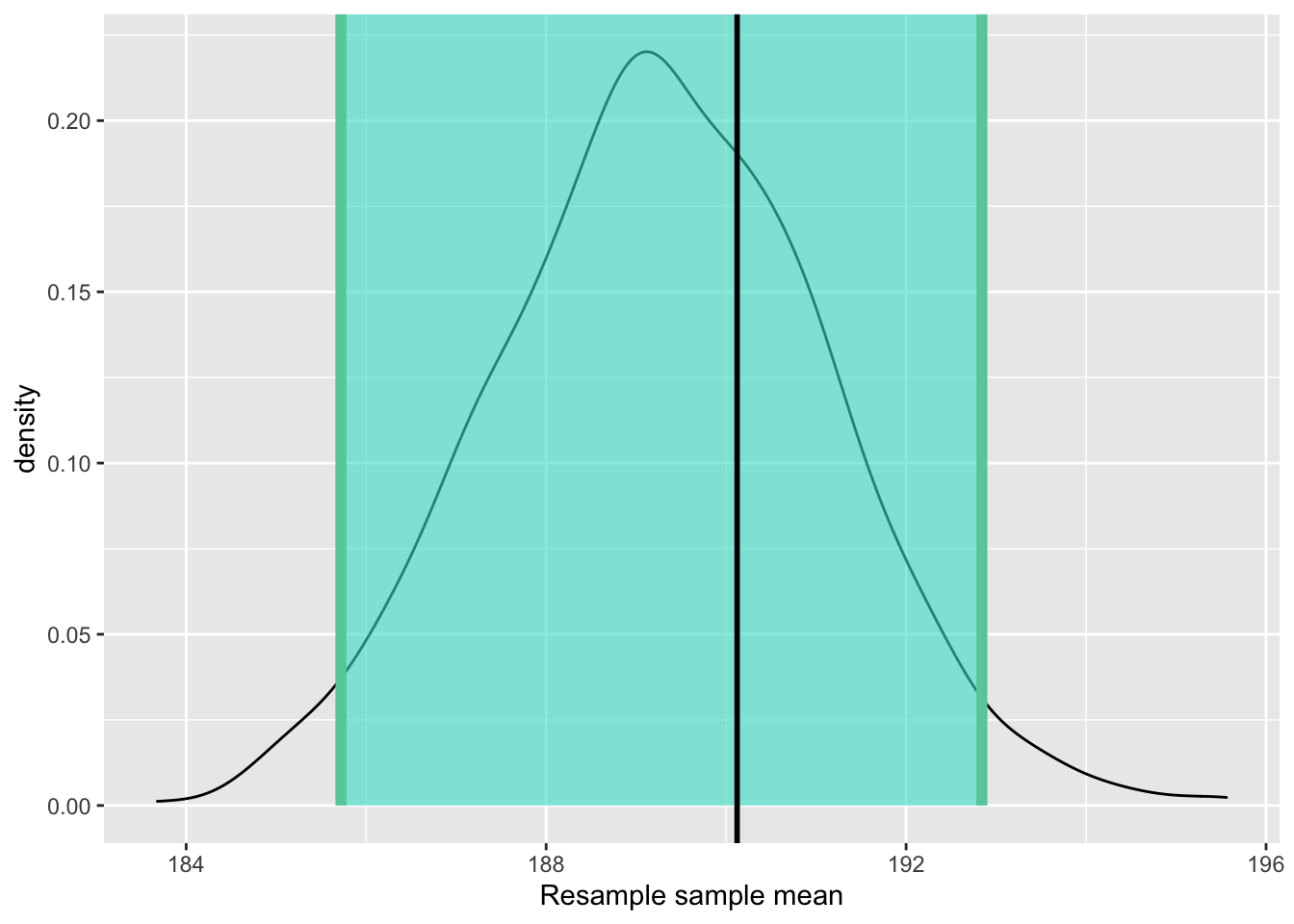
Figure 6.9: Percentile method 95% confidence interval. True population mean marked by a vertical line.

As shown in Figure 6.9, The true value of $\mu$ marked by the black vertical line is well within the confidence interval marked by the turquoise-coloured area. Therefore, we can say that this particular confidence interval did capture the population mean. But was it pure luck that the confidnece interval I construcuted captured the population parameter? Had I had another sample to start with — unbiased and randomly chosen, but different from the previous sample, would it still result in a confidence interval that captures the population mean?

Let’s put this idea to test now that we have access to the entire (simulated) population of bananas. Specifically, let’s draw 100 samples from the population, and construct a bootstrap confidence interval from each sample, which would result in 100 bootstrap confidence intervals.

Let’s visusalize the results in Figure 6.10 where:

We mark the true value of $\mu = 190.12$ with a vertical line.
We mark each of the one-hundred 95% confidence intervals with horizontal lines. These are the “nets.”
The horizontal line is colored grey if the confidence interval “captures” the true value of $\mu$ marked with the vertical line. The horizontal line is colored black otherwise.

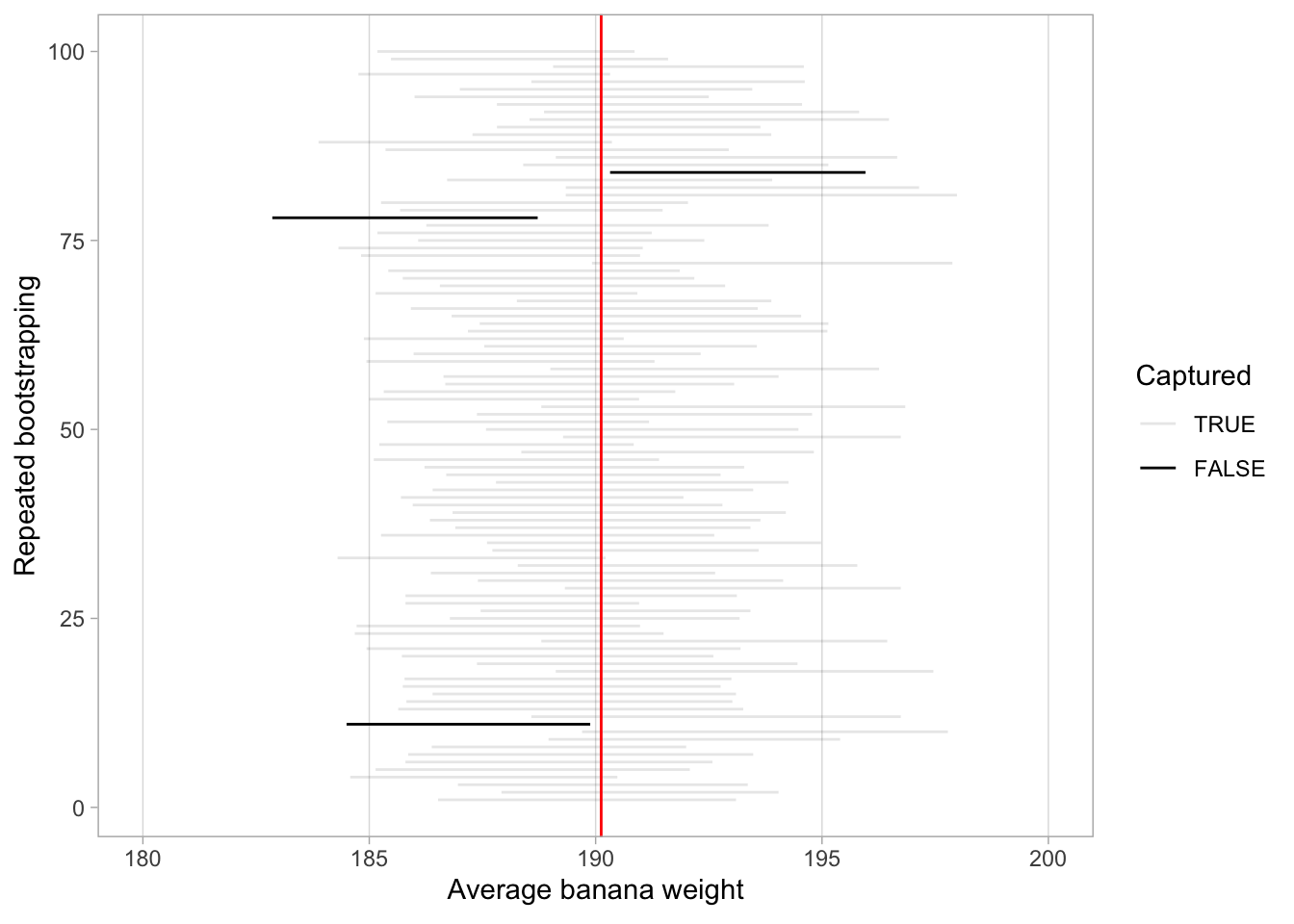
$100 percentile-based 95% confidence intervals for $\mu$.$

Figure 6.10: 100 percentile-based 95% confidence intervals for $\mu$.

Of the one-hundred 95% confidence intervals, 97 of them captured the true value 190.12, whereas 3 of them did not. To apply the fishing analogy again, 100 people cast their net, 97 of them caught fish, whereas 3 of them came back empty. Now is the time to introduce the formal definition of the 95% confidence interval:

For every one hundred 95% confidence intervals, we expect that 95 of them will capture the population quantity (e.g., $\mu$) and that five of them won’t.

Note that “expect” is a probabilistic statement referring to a long-run average. In other words, for every 100 confidence intervals, we will observe about 95 confidence intervals that capture the population parameter, but not always exactly 95. In Figure 6.10 for example, 97 of the confidence intervals captured $\mu$.

To further accentuate the point about confidence levels, let’s generate a figure similar to Figure 6.10, but this time constructing 80% confidence intervals instead. Let’s visualize the results in Figure 6.11 with the scale on the x-axis being the same as in Figure 6.10 to make comparison easy.

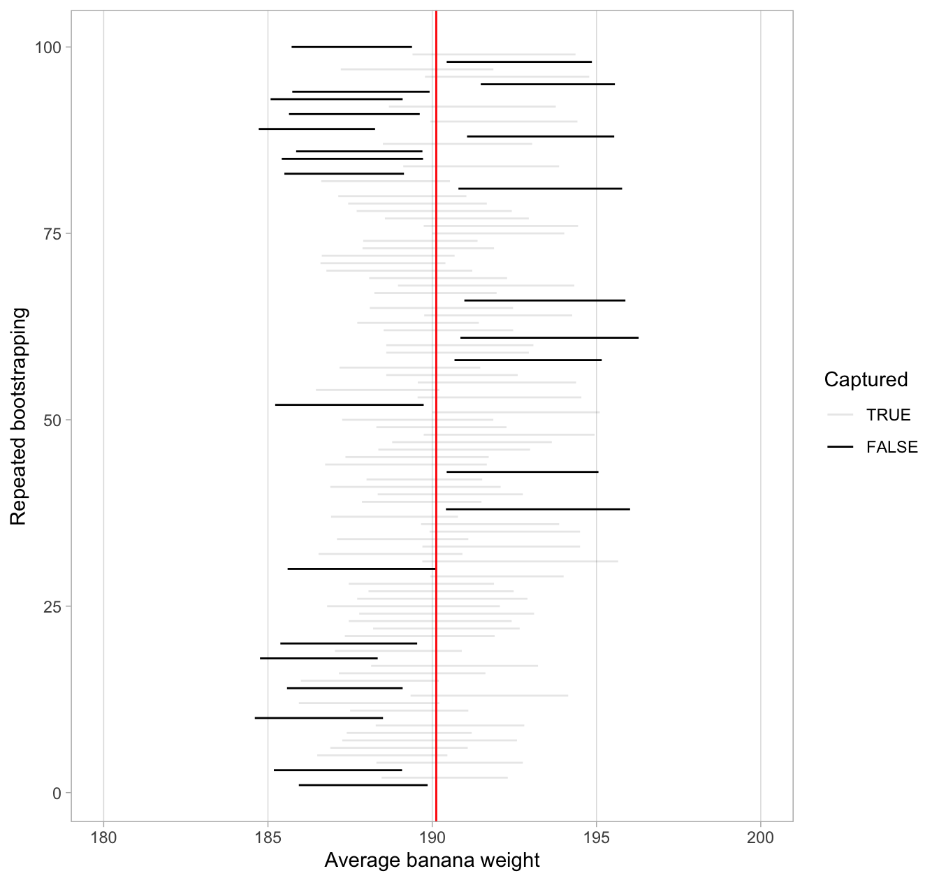
$100 percentile-based 80% confidence intervals for $\mu$.$

Figure 6.11: 100 percentile-based 80% confidence intervals for $\mu$.

Observe how the 80% confidence intervals are narrower than the 95% confidence intervals. Consider the size of the confidence interval as the size of a net. The smaller the size, the lower chance that this net will catch the target. We will explore other determinants of condidence interval width in the upcoming section 6.6.3.

Furthermore, observe that of the one-hundred 80% confidence intervals, 75 of them captured the population mean weight $\mu$ = 190.12, whereas 25 of them did not. Since we lowered the confidence level from 95% to 80%, we now have fewer confidence intervals that caught the fish.

6.6.2 Precise and shorthand interpretation

Let’s return our attention to 95% confidence intervals. The precise and mathematically correct interpretation of a 95% confidence interval is a little long-winded:

Precise interpretation: If we repeated our sampling procedure a large number of times, we expect about 95% of the resulting confidence intervals to capture the value of the population parameter.

This is what we observed in Figure 6.10. Our confidence interval construction procedure is 95% reliable. That is to say, we can expect our confidence intervals to include the true population parameter about 95% of the time.

A common but incorrect interpretation is: “There is a 95% probability that the confidence interval contains $\mu$.” Looking at Figure 6.10, each of the confidence intervals either does or doesn’t contain $\mu$. In other words, the probability is either a 1 or a 0.

Loosely speaking, we can think of these intervals as our “best guess” of a plausible range of values for the mean weight $\mu$ of all bananas. For the rest of this class, we’ll use the following shorthand summary of the precise interpretation.

Short-hand interpretation: We are 95% “confident” that a 95% confidence interval captures the value of the population parameter.

We use quotation marks around “confident” to emphasize that while 95% relates to the reliability of our confidence interval construction procedure, ultimately a constructed confidence interval is our best guess of an interval that contains the population parameter. In other words, it’s our best net.

So returning to our banana weight example and focusing on the percentile method, we are 95% “confident” that the true mean weight of bananas is somewhere between 185.72 and 192.84 grams.

6.6.3 Width of confidence intervals

Impact of confidence level

One factor that determines confidence interval widths is the pre-specified confidence level. For example, in Figures 6.10 and 6.11, we compared the widths of 95% and 80% confidence intervals and observed that the 95% confidence intervals were wider. In order to be more confident in our best guess of a range of values, we need to widen the range of values.

To elaborate on this, imagine we want to guess the forecasted high temperature in Ottawa, Canana on May 15th. Given Ottawa’s temperate climate with four distinct seasons, we could say somewhat confidently that the high temperature would be between 10°C - 20°C. However, if we wanted a temperature range we were absolutely confident about, we would need to widen it.

We need this wider range to allow for the possibility of anomalous weather, like a freak cold spell or an extreme heat wave. So a range of temperatures we could be near certain about would be between 0°C - 35°C. On the other hand, if we could tolerate being a little less confident, we could narrow this range to between 10°C - 20°C.

In order to have a higher confidence level, our confidence intervals must be wider. Ideally, we would want a high confidence level and a narrow confidence intervals. However, we cannot have it both ways. If we want to be more confident, we need to allow for wider intervals. Conversely, if we would like a narrow interval, we must tolerate a lower confidence level.

The moral of the story is: Holding everything else constant, higher confidence levels tend to produce wider confidence intervals. When looking at Figure 6.10 and Figure 6.11, it is important to keep in mind that we kept the sample size fixed at $n$ = 50. What happens if instead we took samples of different sizes?

Impact of sample size

This time, let’s fix the confidence level at 95%, but consider three different sample sizes for $n$: 25, 50, and 100. Specifically, we’ll take 30 different random samples — 10 random samples of size $n = 25$, 10 random samples of size $n = 50$, and 10 random samples of size $n = 100$. We’ll then construct 95% percentile-based confidence intervals for each sample. Finally, we’ll compare the widths of these intervals. We visualize the resulting 30 confidence intervals in Figure 6.12. Note also the vertical line marking the true value of $\mu$ = 190.12.

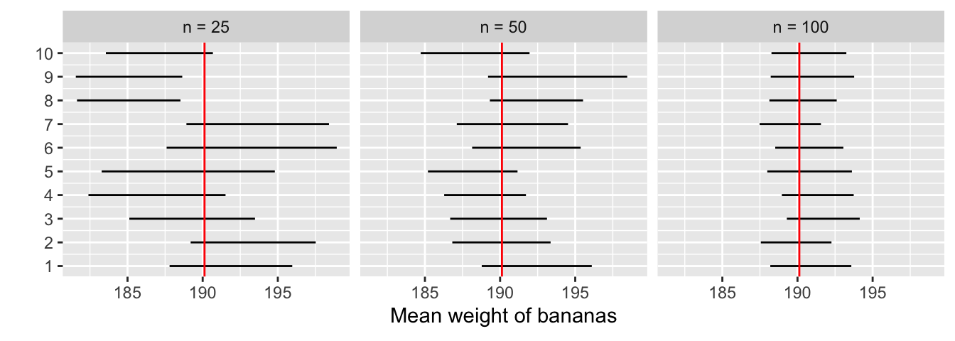
$Ten 95% confidence intervals for $\mu$ with $n = 25, 50,$ and $100$.$

Figure 6.12: Ten 95% confidence intervals for $\mu$ with $n = 25, 50,$ and $100$.

Observe that as the confidence intervals are constructed from larger and larger sample sizes, they tend to get narrower. Let’s compare the average widths in Table 6.2.

Table 6.2: Average width of 95% confidence intervals based on $n = 25$, $50$, and $100$
Sample size	Mean width
n = 25	8.738
n = 50	6.903
n = 100	4.898

The moral of the story is: Larger sample sizes tend to produce narrower confidence intervals. The bigger the sample size, the narrower the confidence interval, and thus the smaller the expected uncertainty in the estimated population parameter. This is why you sometimes hear the notion that a bigger sample size is preferable (within reasonable limits). A bigger sample size allows you to get a more precise estimate of the population parameter.

Impact of standard deviation

Recall that, using the theory-based method, the confidence interval can be estimated via Equation (6.2). I reproduce the equation below:

\[ \bar{x} \pm (1.96 \cdot SE_\bar{x}) = \bar{x} \pm (1.96 \cdot \frac{sd}{\sqrt{n}}) \]

Based on this equation, the width of the a confidence interval is tied to three factors: the multiplier (e.g., 1.96), or the confidence level; the sample size (e.g., n = 50); and the sample standard deviation.

We have shown that the width of a confidence interval increases as the confidence level / multiplier increases, and that it decreases as the sample size increases (because $\sqrt{n}$ is in the denominator). Likewise, the larger the sample standard deviation, the wider the confidence interval.

To summarize, confidence interval widths are determined by an interplay of the confidence level, the sample size n, and the standard deviation.

6.7 Conclusion

6.7.1 Constructing confidence intervals with package `infer`

In Section 6.3.2, we used the infer::rep_sample_n() function to generate 1,000 REsamples with replacemen. In this section, we will build off that idea to construct bootstrap confidence intervals using a new package infer. This pacakge provides functions with intuitive verb-like names to perform statistical inferences. It makes efficient use of the %>% pipe operator to spell out the sequence of steps necessary to perform statistical inference. Let’s now illustrate the sequence of verbs necessary to construct a confidence interval for $\mu$, the population mean weight of bananas.

1. `specify` variables

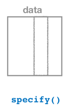
Figure 6.13: Diagram of the specify() verb.

As shown in Figure 6.13, the specify() function is used to choose which variables in a data frame will be the focus of our statistical inference. We do this by specifying the response argument. For example, in our banana_sample data frame of the 50 bananas, the variable of interest is weight:

banana_sample %>% 
  infer::specify(response = weight)

Response: weight (numeric)
# A tibble: 50 x 1
   weight
    <dbl>
 1    209
 2    210
 3    186
 4    184
 5    205
 6    182
 7    184
 8    183
 9    175
10    183
# … with 40 more rows

2. `generate` replicates

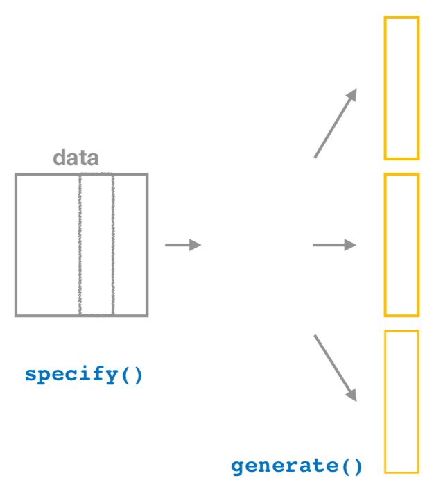
Figure 6.14: Diagram of generate() replicates.

After we specify() the variables of interest, we pipe the results into the generate() function to generate replicates. Figure 6.14 shows how this is combined with specify() to start the pipeline. In other words, repeat the resampling process a large number of times. Recall in Sections 6.3.2 we did this 1000 times.

The generate() function’s first argument is reps, which sets the number of replicates we would like to generate. Since we want to resample the 50 bananas in banana_sample with replacement 1000 times, we set reps = 1000. The second argument type determines the type of computer simulation we’d like to perform. We set this to type = "bootstrap" indicating that we want to perform bootstrap resampling. You’ll see different options for type in Chapter 7.

banana_sample %>% 
  infer::specify(response = weight) %>% 
  infer::generate(reps = 1000, type = "bootstrap")

Response: weight (numeric)
# A tibble: 50,000 x 2
# Groups:   replicate [1,000]
   replicate weight
       <int>  <dbl>
 1         1    183
 2         1    175
 3         1    183
 4         1    209
 5         1    184
 6         1    198
 7         1    186
 8         1    210
 9         1    173
10         1    183
# … with 49,990 more rows

Observe that the resulting data frame has 50,000 rows. This is because we performed resampling of 50 bananas with replacement 1000 times and 50,000 = 50 $\cdot$ 1000.

The variable replicate indicates which resample each row belongs to. So it has the value 1 50 times, the value 2 50 times, all the way through to the value 1000 50 times. The default value of the type argument is "bootstrap" in this scenario, so if the last line was written as generate(reps = 1000), we’d obtain the same results.

Comparing with original workflow: Note that the steps of the infer workflow so far produce the same results as the original workflow using the rep_sample_n() function we saw earlier. In other words, the following two code chunks produce similar results:

# infer workflow:                            # Original workflow:
banana_sample %>%                            banana_sample %>% 
  infer::specify(response = weight) %>%        infer::rep_sample_n(size = 50, replace = TRUE, 
  infer::generate(reps = 1000)                                     reps = 1000)

3. `calculate` summary statistics

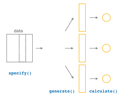
Figure 6.15: Diagram of calculate() summary statistics.

After we generate() many replicates of bootstrap resampling with replacement, we next want to summarize each of the 1000 resamples of size 50 to a single sample statistic value. As seen in the diagram, the calculate() function does this.

In our case, we want to calculate the mean weight for each bootstrap resample of size 50. To do so, we set the stat argument to "mean". You can also set the stat argument to a variety of other common summary statistics, like "median", "sum", "sd" (standard deviation), and "prop" (proportion). To see a list of all possible summary statistics you can use, type ?infer::calculate and read the help file.

Let’s save the result in a data frame called bootstrap_distribution and explore its contents:

bootstrap_distribution <- banana_sample %>% 
  infer::specify(response = weight) %>% 
  infer::generate(reps = 1000) %>% 
  infer::calculate(stat = "mean")
bootstrap_distribution

# A tibble: 1,000 x 2
   replicate   stat
 *     <int>  <dbl>
 1         1 188.14
 2         2 190.42
 3         3 191.08
 4         4 186.16
 5         5 192.82
 6         6 190.62
 7         7 193.2 
 8         8 190.08
 9         9 191.4 
10        10 188.86
# … with 990 more rows

Observe that the resulting data frame has 1000 rows and 2 columns corresponding to the 1000 replicate values. It also has the mean weight for each bootstrap resample saved in the variable stat.

Comparing with original workflow: You may have recognized at this point that the calculate() step in the infer workflow produces the same output as the group_by() %>% summarize() steps in the original workflow.

# infer workflow:                           # Original workflow:
banana_sample %>%                           banana_sample %>% 
  infer::specify(response = weight) %>%        infer::rep_sample_n(size = 50, replace = TRUE, 
  infer::generate(reps = 1000) %>%                                 reps = 1000) %>%              
  infer::calculate(stat = "mean")              dplyr::group_by(replicate) %>% 
                                               dplyr::summarize(stat = mean(weight))

4. `visualize` the results

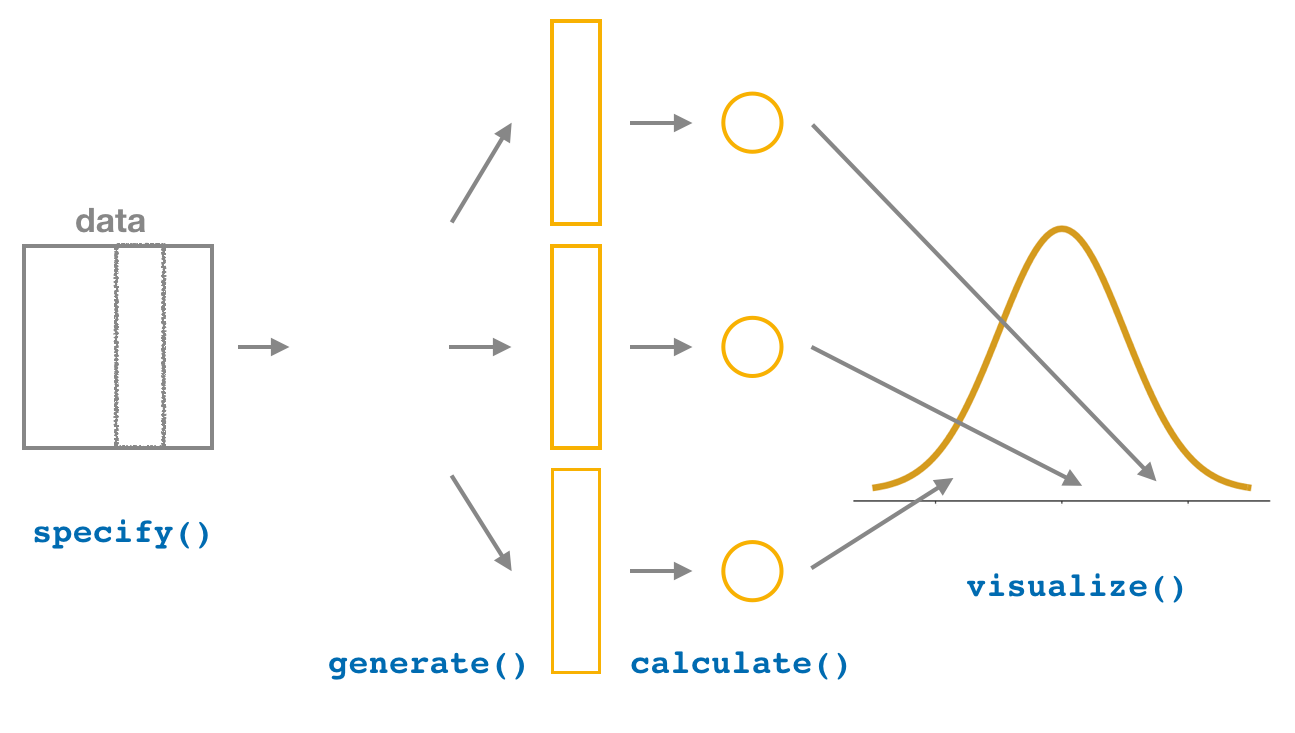
Figure 6.16: Diagram of visualize() results.

The visualize() verb provides a quick way to visualize the bootstrap distribution as a histogram of the numerical stat variable’s values. The pipeline of the main infer verbs used for exploring bootstrap distribution results is shown in Figure 6.16.

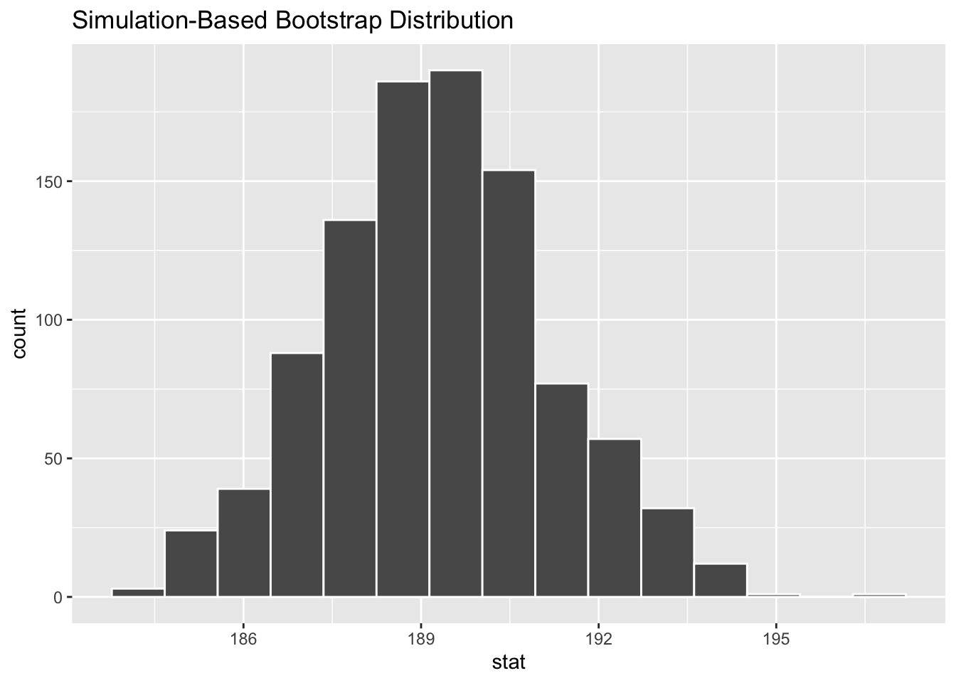
infer::visualize(bootstrap_distribution)

Figure 6.17: Bootstrap distribution.

Comparing with original workflow:

# infer workflow:                           # Original workflow:
infer::visualize(bootstrap_distribution)    ggplot2::ggplot(bootstrap_distribution, 
                                                            ggplot2::aes(x = stat)) +
                                              ggplot2::geom_histogram()

The visualize() function can take many other arguments which we’ll see momentarily to customize the plot further. It also works with helper functions to do the shading of the histogram values corresponding to the confidence interval values.

Let’s recap the steps of the infer workflow for constructing a bootstrap distribution and then visualizing it in Figure 6.18.

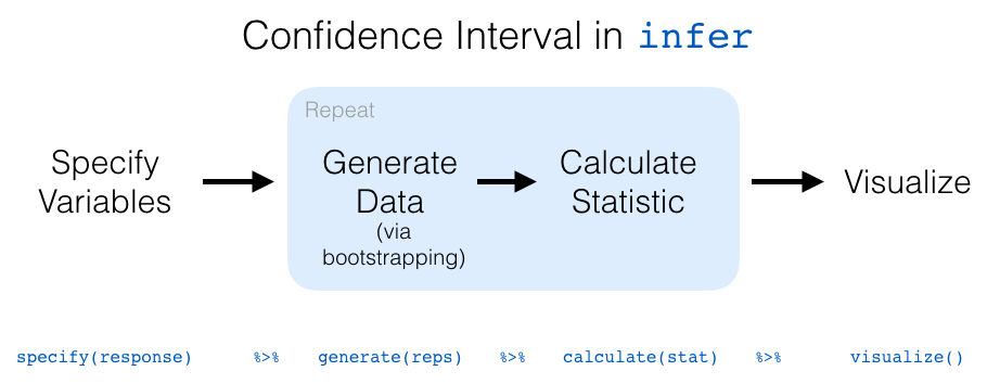
Figure 6.18: infer package workflow for confidence intervals.

Recall how we introduced two different methods for constructing 95% confidence intervals for an unknown population parameter in Section 6.4: the percentile method and the standard error method. Let’s now check out the infer package code that explicitly constructs these. There are also some additional neat functions to visualize the resulting confidence intervals built-in to the infer package!

6.7.2 Percentile method with `infer`

Recall the percentile method for constructing 95% confidence intervals we introduced in Subsection 6.4.1. This method sets the lower endpoint of the confidence interval at the 2.5th percentile of the bootstrap distribution and similarly sets the upper endpoint at the 97.5th percentile. The resulting interval captures the middle 95% of the values of the sample mean in the bootstrap distribution.

We can compute the 95% confidence interval by piping bootstrap_distribution into the get_confidence_interval() function from the infer package, with the confidence level set to 0.95 and the confidence interval type to be "percentile". Let’s save the results in percentile_ci.

percentile_ci <- bootstrap_distribution %>% 
  infer::get_confidence_interval(level = 0.95, type = "percentile")
percentile_ci

# A tibble: 1 x 2
  lower_ci upper_ci
     <dbl>    <dbl>
1   185.54  193.100

Alternatively, we can visualize the interval [185.54, 193.1] by piping the bootstrap_distribution data frame into the visualize() function and adding a shade_confidence_interval() layer. We set the endpoints argument to be percentile_ci.

infer::visualize(bootstrap_distribution) + 
  infer::shade_confidence_interval(endpoints = percentile_ci)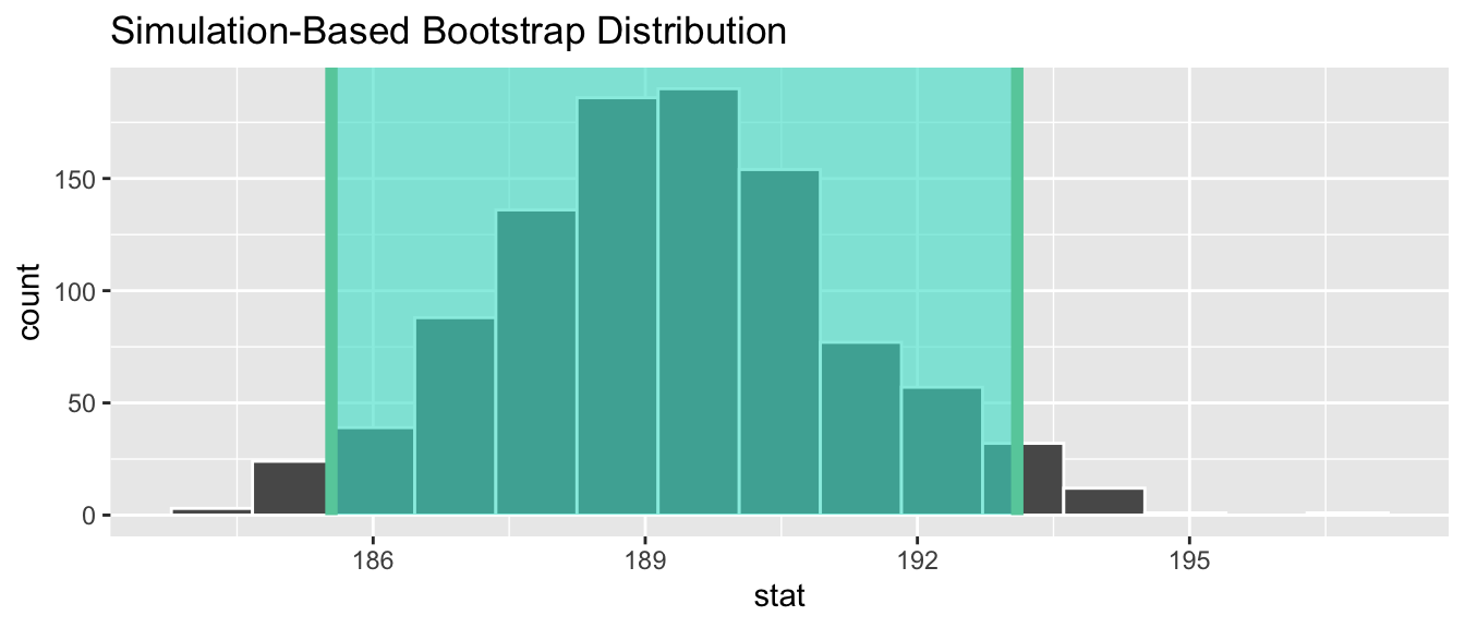

Figure 6.19: Percentile method 95% confidence interval shaded corresponding to potential values.

Observe in Figure 6.19 that 95% of the sample means stored in the stat variable in bootstrap_distribution fall between the two endpoints marked with the darker lines, with 2.5% of the sample means to the left of the shaded area and 2.5% of the sample means to the right. You also have the option to change the colors of the shading using the color and fill arguments.

You can also use the shorter named function shade_ci() and the results will be the same. This is for folks who don’t want to type out all of confidence_interval and prefer to type out ci instead. Try out the following code!

infer::visualize(bootstrap_distribution) + 
  infer::shade_ci(endpoints = percentile_ci, color = "hotpink", fill = "khaki")

6.7.3 Standard error method with `infer`

Recall the standard error method for constructing 95% confidence intervals we introduced in Subsection 6.4.2. For any distribution that is normally shaped, roughly 95% of the values lie within two standard deviations of the mean. In the case of the bootstrap distribution, the standard deviation has a special name: the standard error.

So in our case, 95% of values of the bootstrap distribution will lie within $\pm 1.96$ standard errors of $\bar{x}$. Thus, a 95% confidence interval is

\[ \bar{x} \pm 1.96 \cdot SE = [\bar{x} - 1.96 \cdot SE, \, \bar{x} + 1.96 \cdot SE] \]

Computation of the 95% confidence interval can once again be done by piping the bootstrap_distribution data frame we created into the get_confidence_interval() function. However, this time we set the first type argument to be "se". Second, we must specify the point_estimate argument in order to set the center of the confidence interval. We set this to be the sample mean of the original sample of 50 bananas of 189.3 we have calculated in Section 6.2.

standard_error_ci <- bootstrap_distribution %>% 
  infer::get_confidence_interval(type = "se", point_estimate = m_onesample, level =0.95)
standard_error_ci

# A tibble: 1 x 2
  lower_ci upper_ci
     <dbl>    <dbl>
1  185.570  193.030

If we would like to visualize the interval (185.57, 193.03), we can once again pipe the bootstrap_distribution data frame into the visualize() function and add a shade_confidence_interval() layer to our plot. We set the endpoints argument to be standard_error_ci. The resulting standard-error method based on a 95% confidence interval for $\mu$ can be seen in Figure 6.20.

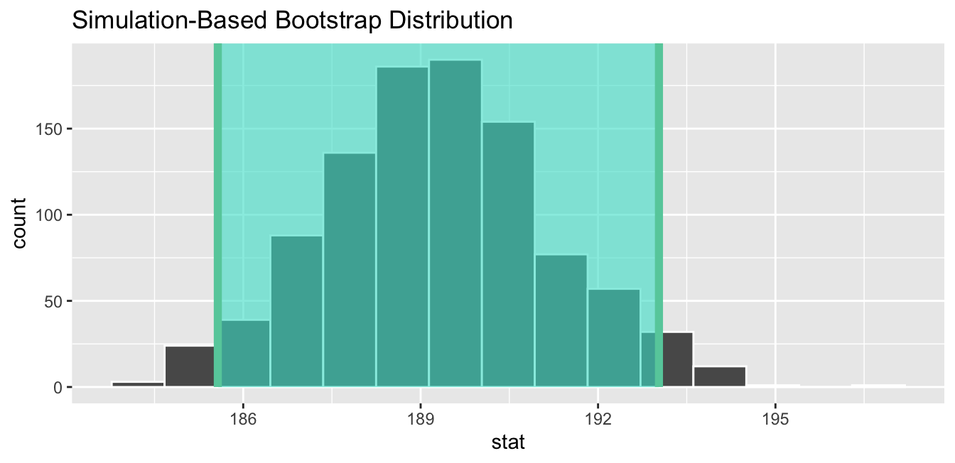
Figure 6.20: Standard-error-method 95% confidence interval.

As noted in Section 6.4, both methods produce similar confidence intervals:

Percentile method: [185.54, 193.1]
Standard error method: [185.57, 193.03]

Learning check

(LC6.1) Construct a 95% confidence interval for the median weight of all bananas. Use the percentile method and, if appropriate, then use the standard-error method.

6.7.4 Comparing bootstrap and sampling distributions

In this chapter, we have learned three methods of constructing confidence intervals. All of them rely on approximating the sampling distribution, either using the Central Limit Theorem, or bootstrap resampling with replacement from a single sample. In the latter case, we used the bootstrap distribution of $\bar{x}$ to approximate the sampling distribution of $\bar{x}$ (Section 6.3.2).

Let’s compare

the sampling distribution of $\bar{x}$ based on 1,000 samples Cy drew from the population banana_pop in Chapter 5, and
the bootstrap distribution of $\bar{x}$ based on 1,000 REsamples with replacement from a single sample banana_samplein Section 6.3.2.

Sampling distribution

Here is the code to construct the sampling distribution of $\bar{x}$ you saw at the beginning of the chapter, reproduced in Figure 6.21, with some changes to incorporate the statistical terminology relating to sampling from Section 5.2.2.

# Take one-thousand samples of size 50 from the population
banana_samples <- banana_pop %>% 
  infer::rep_sample_n(size = 50, reps = 1000, replace = FALSE)

# Compute the sampling distribution of 1000 values of x-bar
sampling_distribution <- banana_samples %>% 
  dp$group_by(replicate) %>% 
  dp$summarize(mean_weight = mean(weight))

# Visualize sampling distribution of x-bar
gg$ggplot(sampling_distribution, gg$aes(x = mean_weight)) + 
  gg$geom_histogram(boundary = 190, binwidth=1, colour="white") + 
  gg$labs(x = "Sample mean weight of 50 bananas (gram)", y = "", 
          title = "Sampling distribution")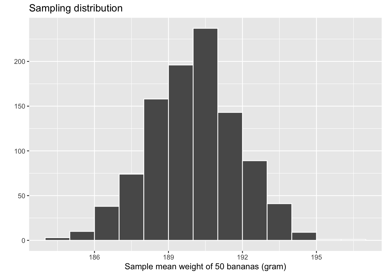

Figure 6.21: Previously seen sampling distribution of sample mean weight for $n = 1000$.

An important thing to keep in mind is the default value for replace is FALSE when using rep_sample_n(). This is because when sampling 50 bananas, we are extracting 50 bananas (i.e., numbers that represent banana weights) from banana_pop all at once. This is in contrast to bootstrap resampling with replacement, where we take one banana weight and put it back before taking the next banana weight.

Let’s quantify the variability in this sampling distribution by calculating the standard deviation of the mean_weight variable representing 1000 values of the sample mean $\bar{x}$. Remember that the standard deviation of the sampling distribution is the standard error, frequently denoted as $SE_{\bar{x}}$.

sampling_distribution %>% dp$summarize(se = sd(mean_weight))

# A tibble: 1 x 1
       se
    <dbl>
1 1.79104

Bootstrap distribution

Here is the code you previously saw in Section 6.7.1 to construct the bootstrap distribution of $\bar{x}$.

bootstrap_distribution <- banana_sample %>% 
  infer::specify(response = weight) %>% 
  infer::generate(reps = 1000, type = "bootstrap") %>% 
  infer::calculate(stat = "mean")

infer::visualize(bootstrap_distribution, boundary=190, binwidth=1, colour="white")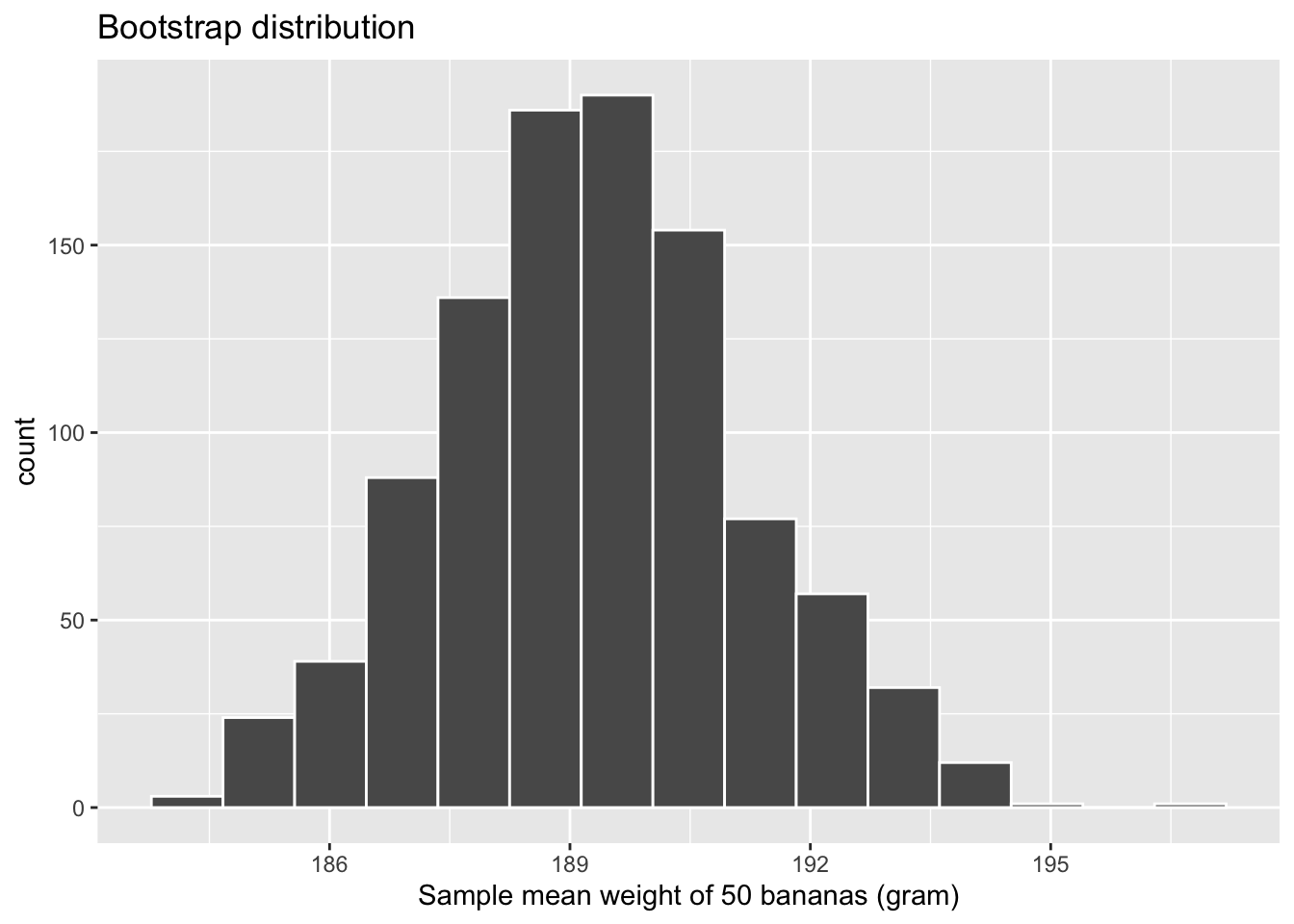

Figure 6.22: Bootstrap distribution of sample mean weight for $n = 1000$.

bootstrap_distribution %>% dp$summarize(se = sd(stat))

# A tibble: 1 x 1
       se
    <dbl>
1 1.90312

Comparison

Now that we have computed both the sampling distribution and the bootstrap distributions, let’s compare them side-by-side in Figure 6.23. We’ll make both histograms have matching scales on the x- and y-axes to make them more comparable. Furthermore, we’ll add:

To the sampling distribution on the top: a solid line denoting the true population mean weight of bananas $\mu = 190.12$.
To the bootstrap distribution on the bottom: a dashed line at the sample mean $\bar{x}$ = 189.3 gram of the original sample banana_sample

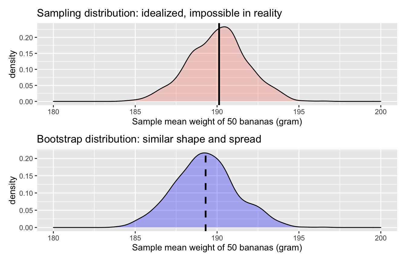
$Comparing the sampling and bootstrap distributions of $\bar{x}$$

Figure 6.23: Comparing the sampling and bootstrap distributions of $\bar{x}$

There is a lot going on in Figure 6.23, so let’s break down all the comparisons slowly. First, observe how the sampling distribution on top is centred at $\mu$ = 190.12. This is because the sampling is done at random and in an unbiased fashion. So the estimates $\bar{x}$ are centred at the true value of $\mu$.

However, this is not the case with the following bootstrap distribution. The bootstrap distribution is centered at 189.3 grams, which is the sample mean weight of banana_sample. This is because we are resampling from the same sample over and over again. Since the bootstrap distribution is centered at the original sample’s mean, it doesn’t necessarily provide a better estimate of $\mu$ = 190.12. This leads us to our first lesson about bootstrapping:

The bootstrap distribution will likely not have the same center as the sampling distribution. In other words, bootstrapping cannot improve the quality of a point estimate.

Second, let’s now compare the spread of the two distributions: they are somewhat similar. In the previous code, we computed the standard deviations of both distributions as well. Recall that such standard deviations have a special name: standard errors. Let’s compare them in Table 6.3.

Table 6.3: Comparing standard errors
Distribution type	Standard error
Sampling distribution	1.791
Bootstrap distribution	1.903

Notice that the bootstrap distribution’s standard error is a rather good approximation to the sampling distribution’s standard error. This leads us to our second lesson about bootstrapping:

Even if the bootstrap distribution might not have the same center as the sampling distribution, it will likely have very similar shape and spread. In other words, bootstrapping will give you a good estimate of the standard error.

Thus, using the fact that the bootstrap distribution and sampling distributions have similar spreads, we can build confidence intervals using bootstrapping as we’ve done all throughout this chapter!

If you want more examples of the infer workflow to construct confidence intervals, we suggest you check out the infer package homepage, in particular, a series of example analyses available at https://infer.netlify.app/articles/.

6.7.5 What’s to come?

Now that we’ve equipped ourselves with confidence intervals, in Chapter 7 we’ll cover the other common tool for statistical inference: hypothesis testing. Just like confidence intervals, hypothesis tests are used to infer about a population using a sample. However, we’ll see that the framework for making such inferences is slightly different.

1.96 standard deviations to be exact. For simplicity, I rounded it up to 2 here.↩︎
Bootstrap is a misnomer?↩︎