Chapter 5 Central Limit Theorem
In this chapter,
we kick off the second portion of this book on statistical inference
by presenting the Central Limit Theorem.
Understanding this theorem is essential to
correctly interpreting a p value or a confidence interval,
which we will cover in Chapters 6
and 7.
Can you, with absolute confidence, explain the difference between
a standard deviation and a standard error?
If not, then you will want to read this chapter read this chapter twice.
Good to know
Theorem vs. Theory
From Wikipedia:
In mathematics, a theorem is a … statement that has been proven to be true, either on the basis of generally accepted statements such as axioms or on the basis of previously established statements such as other theorems. A theorem is hence a logical consequence of the axioms, with a proof of the theorem being a logical argument which establishes its truth through the inference rules of a deductive system.
Theorems in mathematics and theories in science are fundamentally different in their epistemology. A scientific theory cannot be proved; its key attribute is that it is falsifiable, that is, it makes predictions about the natural world that are testable by experiments. Any disagreement between prediction and experiment demonstrates the incorrectness of the scientific theory, or at least limits its accuracy or domain of validity. Mathematical theorems, on the other hand, are purely abstract formal statements: the proof of a theorem cannot involve experiments or other empirical evidence in the same way such evidence is used to support scientific theories.
5.1 Meet Central Limit Theorem
Central Limit Theorem is ubiquitous in statistics textbooks, because it is fundamental to inferential statistics. Understanding the theorem requires a thought experiment which, until very recently, is head-scratching, to put it mildly. Thanks to the cheap computing power now at our disposal, we do not have to rely solely on our imagination. We can show and tell!
Next, I present the theorem in steps. At each step, I will illustrate the theorem with simulated data.
5.1.1 Many samples
If you take a large number of samples from a population, compute the sample mean from each sample, then the distribution of the sample means will be approximately normally distributed.
This part of Central Limit Theorem involves two actions: take … samples, and compute the sample mean from each sample.
Most of you are likely already familiar with the process of “taking one sample from a population.” Whether you recruit 30 people for a lab experiment or survey 100 people for an online questionnaire, in each case, you are taking one sample from a population. To honour my “show-and-tell” promise, let’s now simulate the process of “taking one sample from a population.”
Cy was just named the chief statistician in The People’s Republic of Banana. And her country has recently gained independence after a long fought battle. As a result of the new freedom, her country now owns all bananas that exist or will exist in the world. Feeling triumphant, she decided that her first mission would be to study the weight of bananas.
She starts by taking one sample of 50 bananas, measuring the weight of each, and plotting their weights.
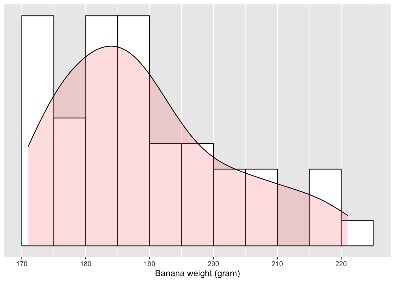
Figure 5.1: Distribution of 50 bananas’ weight
Eyeballing the distribution of these 50 bananas’ weight, Cy learned the following:
1. Not all bananas in her sample weigh the same; some are heavier than others.
2. Despite their weight difference, they don’t differ wildly; most bananas in Cy’s sample weigh between 150 to 250 grams.
3. The distribution of weights is right-skewed.
With a little more effort, Cy also calculated the average weight of the 50-banana sample:
4. In her sample, the bananas weigh 189 grams on average.
We have simulated the process of “taking one sample.” The premise of Central Limit Theorem is to “take a large number of samples.” This is equivalent to repeating the aforementioned banana experiment many times. Let’s continue our show-and-tell.
Cy is not convienced that she has thoroughly studied the banana weight. Next, she is going to repeat the previous process 1,000 times: randomly sample 50 bananas, weigh them, calculate the mean weight, randomly sample another 50 bananas, so on and so forth. Each repeat, Cy will use randomly chosen bananas, rather than weighing the same 50 bananas over and over. Of course, it will likely take her a long time to complete these repetitions, but as the new nation’s chief statistician, she feels obligated to give her best effort to this important matter.
After days’ hardwork, Cy completed weighing and plotting 1,000 banana samples.
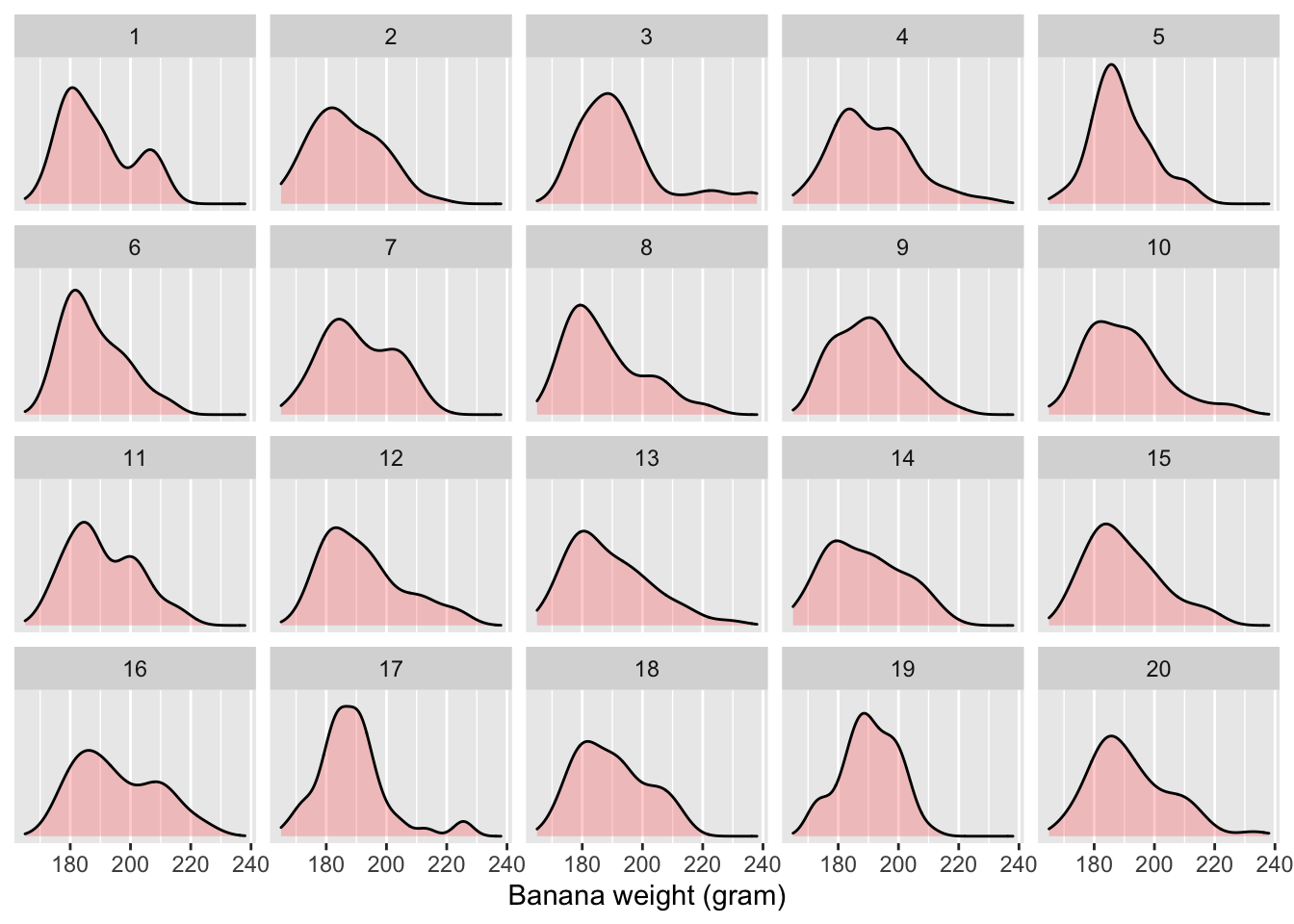
Figure 5.2: Distribution of 50 bananas’ weight in the first 20 samples out of 1,000
| replicate | Average Weight |
|---|---|
| 1 | 189 |
| 2 | 187 |
| 3 | 192 |
| 4 | 191 |
| 5 | 189 |
| 6 | 188 |
| 7 | 191 |
| 8 | 187 |
| 9 | 190 |
| 10 | 190 |
| 11 | 191 |
| 12 | 192 |
| 13 | 189 |
| 14 | 188 |
| 15 | 190 |
| 16 | 196 |
| 17 | 189 |
| 18 | 190 |
| 19 | 190 |
| 20 | 192 |
In total, Cy drew 1,000 samples of bananas, each containing 50 randomly chosen bananas. With each sample, Cy was able to plot the distribution of their weights and calculate the sample mean. Figure 5.2 visualizes the first 20 of those 1,000 samples. Table 5.1 lists the corresponding sample means for those 20 sample. Eyeballing these distributions and the sample means, Cy learned the following:
1. The distributions in Figure 5.2 look similar to each other, and yet are distinguishable from one another, confirming that 1,000 unique samples were taken from the population.
2. The sample means in Table 5.1 are close to each other in magnitude, but are not all the same.
Having completed both “take a large number of samples” and “compute the sample mean from each sample,” it is time to revisit the Central Limit Theorem.
If you take a large number of samples from a population, compute the sample mean from each sample, then the distribution of the sample means will be approximately normally distributed.
It seems that the next step would be plotting the sample means from those 1,000 samples.
It is hard to discern any pattern by looking at individual numbers in Table 5.1. Cy’s statistical intuition tells her that she should visualize them using a histogram.
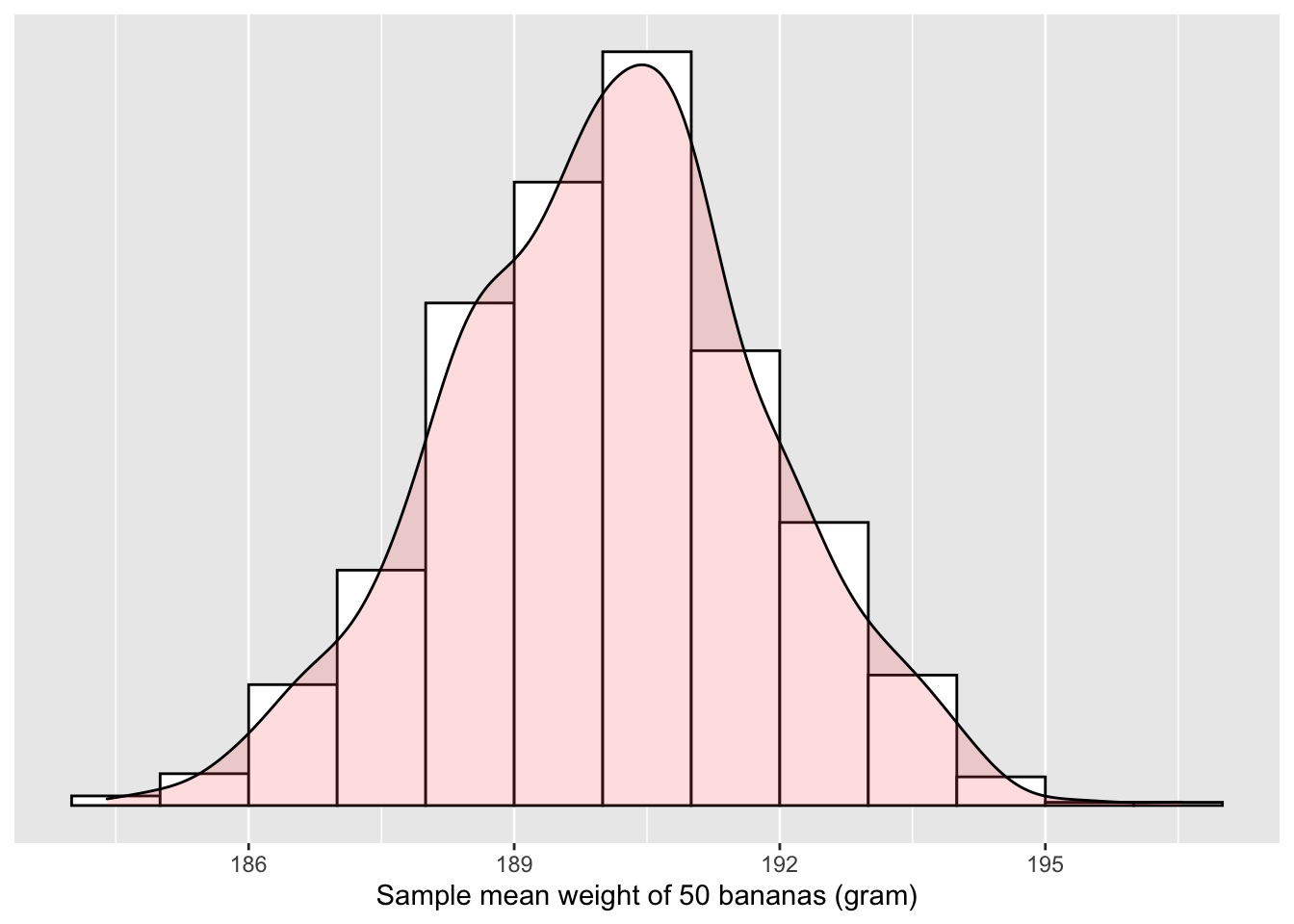
Figure 5.3: Distribution of 1,000 sample means
As a comparison, Cy also decided to place side by side a histogram based on 50 individual bananas and the new histogram based on 1,000 samples means.
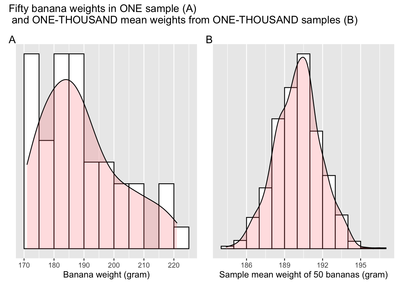
Figure 5.4: A sample distribution and a sampling distribution
Once panel A and B in Figure 5.4 are juxtaposed, the contrast is very telling:
- The distribution of the weight for a single sample is skewed.
- The distribution of the average weight from one-thousand samples is symmetric and resembles that of a normal bell curve.
Just as predicted by the Central Limit Theorem,
If you take a large number of samples from a population, compute the sample mean from each sample, then the distribution of the sample means will be approximately normally distributed.
5.1.2 Sample size
The Central Limit Theorem continues:
This will hold true regardless of whether the source population is normal or skewed, provided the sample size is sufficiently large (usually n > 30). If the population is normal, then the theorem holds true even for samples smaller than 30.
In the simulated banana example we have seen so far, each individual sample shows some skewness (Figure 5.1, Figure 5.2), indicating that the population of banana weight is likely skewed as well. And yet, when the 1,000 sample means were plotted, they conform to a symmetric, bell-like distribution (Figure 5.3. This is not a coincidence or a miracle. It is simply the result of meeting the condition of the Central Limit Theorem, that each sample we drew had a sufficiently large size — 50.
In reality, one can rarely be certain that the population is normally distributed. As a result, we deny ourselves the benefit of doubt, and abide by the rule of thumb that the sample size be larger than 30.
5.1.3 Inference
The Central Limit Theorem continues:
We can make inferences about a population mean and quantify the uncertainty of such inferences based on the sample mean and sample standard deviation.
If you have been wondering why we should bother studying the Central Limit Theorem, this last part of the theorem reveals the reason. The Central Limit Theorem prescribes one way to make inferences. The act of “inferring” in this context means to generalize what we have learned from specific cases to more general cases, guided by laws of statistics. From wikipedia:
[Statistical inference] is the "process of using data analysis to … infer properties of a population, for example by testing hypotheses and deriving estimates. Inferential statistics can be contrasted with descriptive statistics. Descriptive statistics is solely concerned with properties of the observed data, and it does not rest on the assumption that the data come from a larger population.
Research is almost never about a sample, but the population that the sample represents. Whether the target of a research is a correlation, a regression coefficient, or a group difference, it is the correlation, the regression coefficient, or the group difference in the population that we are interested in. What researchers learn from the sample can only be generalized to the population using inferences.
Next, I will demonstrate how to make inferences using the Central Limit Theorem for one particular type of question: estimating the population mean.
After thoroughly examining 1,000 samples and their average weights, Cy estimates that a typical banana weighs 190 grams, and that this estimate has a margin of error of 3.51 grams.
In reality, most of us can only afford the time and resources to study one sample, instead of one-thousand samples. The last part of the Central Limit Theorem assures us that, taking a single sample, and using sample statistics derived from the said sample, allows us to infer the same population mean obtained by Cy, who took a thousand samples.
The Central Limit Theorem further dictates that:
\[ \mu \approx \bar{x} \tag{5.1} \]
The Greek letter \(\mu\) is pronounced mu, sometimes writen as \(\mu_{x}\), and represents the population mean. \(\bar{x}\) is pronounced eks bar, and represents the sample mean. Loosely translated to plain English, Equation (5.1) tells us that the average calculated from one sample is as good as the average calculated from a thousand samples, provided that the first said sample is randomly chosen and is sufficiently large (n > 30). Or in technical terms, sample mean is an unbiased point estimate of population mean.
Finally, the Central Limit Theorem states that:
\[ \sigma_\bar{x} \approx \frac{sd}{\sqrt{n}} \tag{5.2} \] where \(sd\) is the sample standard deviation
The Greek leter \(\sigma\) is pronounced sigma. \(\sigma_\bar{x}\) is pronounced sigma eks bar, and represents the standard deviation of \(\bar{x}\). Equation (5.2) tells us that we can quantify the uncertainty of our estimate in Equation (5.1), by taking the sample standard deviation and dividing it by the square root of sample size.
To understand Equation (5.2), consider its context. As previously mentioned, Equation (5.1) assures that a sample mean is an unbiased point estimate of the population mean. An estimate is not bad, but still is an estimate, an educated guess. To ameliorate the lack of accuracy, statisticians often provide a range that quantifies the uncertainty. For instance, Cy could say that by estimate, a typical banana weighs 190 grams, and I am 95% confident that the average weight of bananas is within 190 \(\pm\) 3.51 grams, or within [186.55, 193.57] grams. Naturally, the wider the range, the higher uncertainty. To say that tomorrow’s high temperature is within the range of -10 to +10°C sounds much more uncertain than to say it is between 0 to 5°C.
Given that a sample mean is merely an estimate of the population mean, how do we dertermine the degree of uncertainty for this estimate? Or what is the size of the range that quantifies the uncertainty? According to Equation (5.2), we could infer the quantity based on the sample standard deviation. In plain English, Equation (5.2) tells us that the uncertainty of our estimated average is proportional to how much values vary within one sample, captured by the sample standard deviation \(sd\), and inversely proportional to the size of each sample, hence \(\sqrt{n}\) in the denominator. We can expect that the sample mean to vary from one sample to the next much less compared to how individual values vary within one sample, roughly by a ratio of \(\sqrt{n}\).
Thus far, we have unpacked the entire Central Limit Theorem. Let’s wrap up by revisiting the theorem and elaborating on key concepts involved in the theorem.
5.2 Revisit the Central Limit Theorem
If you take a large number of samples from a population, compute the sample mean from each sample, then the distribution of the sample means will be approximately normally distributed. This will hold true regardless of whether the source population is normal or skewed, provided the sample size is sufficiently large (usually n > 30). If the population is normal, then the theorem holds true even for samples smaller than 30. We can make inferences about a population mean and quantify the uncertainty of such inferences based on the sample mean and sample standard deviation.
\[ \mu \approx \bar{x} \]
\[ \sigma_\bar{x} \approx \frac{sd}{\sqrt{n}} \]
where \(sd\) is the sample standard deviation
5.2.1 Sample vs. sampling distribution
Figure 5.4 showed two distributions: a distribution of banana weights in ONE sample, and a distribution of 1,000 means weights from ONE-THOUSAND samples. Aside from the fact that the two distributions differ in shape, they also differ in the extent of dispersion, AKA standard deviation (see A.1.3 for a refresher of the concept).
In Figure 5.5, I have reproduced Figure 5.4. In addition, I also marked the one standard deviation above / below the sample average on each distribution.
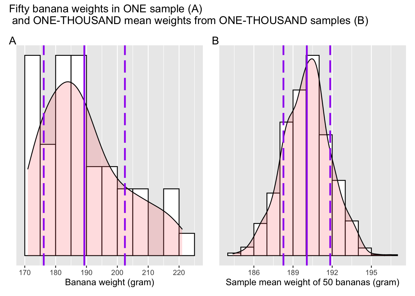
Figure 5.5: Sample and sampling distribution
Can you visually estimate the standard deviation in both distributions, i.e., the distance between a dashed line and the solid line? Note that the scales of the x-axis are different in A and B. In A, either dashed line is about 10 grams apart from the center solid line; in B they are about 1.5 grams apart. Obviously, the distribution in Panel A has a bigger standard deviation than that in Panel B. Their size difference is not a coincidence, but rather prescribed by the Central Limit Theorem. Recall equation (5.2), which states \(\sigma_\bar{x} \approx \frac{sd}{\sqrt{n}}\). \(sd\) is the symbol of sample standard deviation, which is represented by the distance between a dashed line and the solid line in Panel A. \(\sigma_\bar{x}\) is represented by the distance between a dashed line and the solid line in Panel B. Equation (5.2) tells us that \(\sigma_\bar{x}\) is approximately equal to \(sd\) divided by \(\sqrt{n}\). Substitute n with 50, the number of bananas in a sample, which gives us \(\sqrt{n} \approx 7\). In another word, \(\sigma_\bar{x}\) is about one seventh of \(sd\), matching our visual observation (\(1.5 \times 7 \approx 10\)).
Panel A of Figure 5.5 is called a sample distribution whereas Panel B a sampling distribution. The word sampling is used to emphasize how a sampling distribution typically arises: via the repeated action of sampling, computing the average of each resulting sample, and plotting the averages. As was mentioned earlier, the metric of dispersion is generally known as standard deviation. For a sample distribution, the name remains standard deviation, or sample standard deviation, to be precise. For a sampling distribution, however, a special name, standard error of the mean, is often used in place of a generic “standard deviation.”
The word error in standard error of mean is used to conjure up the image of margin of error when approximating the population mean with a sample mean. Such an approximation has its margin of error, the range of which can be quantified with standard error of the mean. We will discuss the concept of margin of error in the following chapter.
According to Equation (5.2) of the Central Limit Theorem, a standard error of the mean, \(\sigma_\bar{x}\), is always a fraction of the sample standard deviation, \(sd\). Note that standard error of mean is often shortened as Standard Error, or \(SE_{\bar{x}}\). Therefore, Equation (5.2) could also be expressed as:
\[ SE_{\bar{x}} \approx \frac{sd}{\sqrt{n}} \tag{5.3} \]
Using Equation (5.3) from the Central Limit Theorem to approximate \(SE_{\bar{x}}\) is considered a theoretical approach, whereas Cy’s method, i.e., panel B of Figure 5.5, is considered empirical, because it involves repeated sampling (1,000 times in this case).
Learning check
(LC5.1) Calculate \(SE_{\bar{x}}\) using both methods by following the code below and compare the results.
# retrieve a single sample of bananas
banana_sample <- dget("https://raw.githubusercontent.com/chunyunma/baby-modern-dive/master/data/banana_sample.txt")
# take a look at the sample
head(banana_sample)
# sample size is 50
n <- 50
# compute standard deviation for the single sample
sd_onesample <- banana_sample %>%
dplyr::summarize(sd = sd(weight))
# estimate standard error using Equation (5.3)
se_theory <- sd_onesample / sqrt(n) %>% round(2)
se_theory# retrieve the 1,000 sample means
banana_sample_means <- dget("https://raw.githubusercontent.com/chunyunma/baby-modern-dive/master/data/banana_sampling_ch5.txt")
# take a look at the sample means
head(banana_sample_means)# compute standard deviation for the sampling distribution,
# aka, the standard error
se_empirical <- dplyr::summarize(banana_sample_means, sd(mean_weight)) %>%
round(2)
se_empiricalHow does se_theory compare to se_empirical?
5.2.2 More terminology and notations
Here is a list of concepts instrumental to understanding the Central Limit Theorem.
It is okay if you are not familiar with them yet.
We will repeat, clarify these definitions as we move along the course.
A population is a collection of individuals or observations we are interested in. This is also commonly denoted as a study population. We mathematically denote the population’s size using upper-case \(N\). Strictly speaking, the (study) population in Cy’s banana study is the measurable banana weights from all bananas that exist, not the bananas. However, in practice, we often use them interchangeably. We can consider the population’s size \(N\) infinitely large, or unknown, as in many other cases, although there are cases where you could find out the population’s size, such as the (quite literally) population size of a country.
A sample is a subset of a target population, selected via a defined procedure from the population. A sample is said to be a representative sample if it roughly looks like the population.
An unbiased sample is where every observation in a population had an equal chance of being sampled. An unbiased sample is sometimes called a random sample, in that we sample randomly from the population in an unbiased fashion.Sampling is the act of collecting a sample from the population when we don’t have the means to examine every entity in the population, also known as a census. We mathematically denote the sample’s size using lower case \(n\), as opposed to upper case \(N\) which denotes the population’s size. Typically the sample size \(n\) is much smaller than the population size \(N\). Thus sampling is often a cheaper alternative than performing a census.
A population parameter is a numerical summary quantity about the population that is unknown, but you wish you knew. For example, when this quantity is a mean, the population parameter of interest is the population mean. This is mathematically denoted with the Greek letter \(\mu\) pronounced “mu.” The most common types of population parameters include mean, difference between two means, polled difference among multiple means, and slope of a regression line.
A point estimate (AKA sample statistic) is a summary statistic computed from a sample that estimates an unknown population parameter. We mathematically denote the point estimate based on a sample by placing a “hat” on top of the population parameter. For example, \(b\) and \(\widehat{b}\), \(\mu\) and \(\widehat{\mu}\). However, sometimes people also use \(\bar{x}\) (pronounced “x-bar”) instead of \(\widehat{\mu}\), to represent the sample mean.
We say a sample is generalizable if any results based on the sample can generalize to the population. In other words, does the value of the point estimate generalize to the population? Using our mathematical notation, this is akin to asking if \(\bar{x}\) is a “good guess” of \(\mu\)?
To summarize:
If sampling a sample of size \(n\) is done at random, then
the sample is unbiased and representative of the population of size \(N\) (which may be unknown), thus
any result based on the sample can generalize to the population, thus
the point estimate is a good guess of the unknown population parameter, thus
instead of performing a census, we can infer about the population using sampling.
Specific to Cy’s banana study:
She weighed a sample of \(n=50\) bananas chosen at random, then
the banana weights in her sample are an unbiased representation of the weights of all bananas, thus
any result based on her banana sample can generalize to all bananas, thus
the mean weight \(\widehat{\mu}\) of the \(n=50\) bananas in her sample is a good guess of the population weight \(\mu\) of all banans (\(N = +\infty\)), thus
instead of weighing all bananas (unfeasible in reality), we can infer about the weight of a banana using a sample statistic.
5.3 Conclusion
Thus far, I have walked you through the Central Limit Theorem by applying it to the problem of banana weight. Understanding the logic of the theorem requires a thought experiment, which was acted out by our protagonist Cy. The theorem prescribes how to infer the weight of a typical banana in the population from a sample of bananas. With a randomly chosen sample of bananas, its average weight, 189 grams, is an unbiased estimate of the weight of a typical banana in the population. The uncertainty of this estimate, \(\pm 1.86\) grams, is quantified by the standard deviation of the sampling distribution, commonly known as the standard error of mean. In practice, standard error of mean can be approximated using the sample standard deviation divided by square root of sample size.
The concepts of sampling and standard error that we have seen in this chapter
form the basis of confidence intervals and hypothesis testing,
which we’ll cover in Chapters 6
and 7.
We will see that the tools that you learned in the first portion of this book,
in particular data visualization and data wrangling,
will also play an important role in the development of your understanding.
As mentioned before, the concepts throughout this text
all build into a culmination allowing you to untangle the narrative behind the data.
5.4 P.S.
What inspired my creation of Cy the protagonist in this chapter?
One christmas, we embarked on an endeavour:

Figure 5.6: We bought bananas in bulk
After hours of peeling and slicing:

Figure 5.7: We peeled all the bananas
Long story short, we snacked on home-made dehydrated banana chips for the next 12 months after this grand experiment.